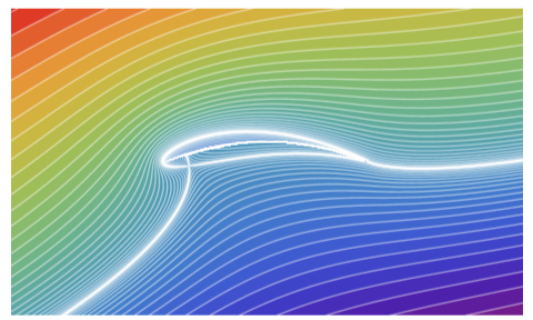
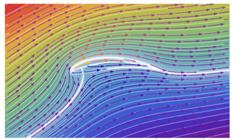
There is no simple method to display streamlines using the Zhukovsky function. I will show an example with a Zhukovsky profile at an angle of attack.
In[]:=
Clear[z];U=rho=1;chord=4;thk=0.5;alpha=Pi/9;y0=0.2;x0=-thk/5.2;L=chord/4;a=Sqrt[y0^2+L^2];gamma=4PiaUSin[alpha+ArcCos[L/a]];w[z_,sign_]:=Module[{zeta=(z+signSqrt[z^2-4L^2])/2},zeta=(zeta-x0-Iy0)Exp[-Ialpha]/Sqrt[(1-x0)^2+y0^2];U(zeta+a^2/zeta)+IgammaLog[zeta]/(2Pi)];sign[z_]:=Sign[Re[z]]If[Abs[Re[z]]<chord/2&&0<Im[z]<2y0(1-(2Re[z]/chord)^2),-1,1];w[z_]:=w[z,sign[z]];V[z_]=D[w[z,sig],z]/.sig->sign[z];bg1=ContourPlot[Im[w[(x+Iy)]],{x,-5,5},{y,-3,3},AspectRatio->Automatic,ColorFunction->"Rainbow",Contours->Table[x^3+0.0208,{x,-2,2,0.05}],ContourStyle->White,PlotPoints->40,Frame->False,Exclusions->{Log[x+Iy]==0}]
Out[]=
In[]:=
J=Show[bg1,StreamPlot[{Re[V[x+Iy]],-Im[V[x+Iy]]},{x,-5,5},{y,-3,3},AspectRatio->Automatic,StreamStyle->LightGray,Frame->False,StreamPoints->Fine]]
Out[]=
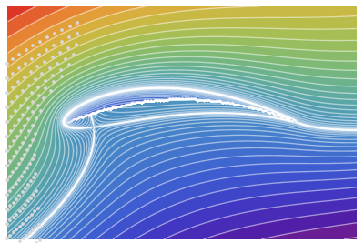
We can add animation for particles carried away by the flow
In[]:=
w1[z_]:=w[z,sign[z]];VX=Evaluate[D[w[z,s],z]/.{z->x+Iy,s->sign[x+Iy]}];bg=ContourPlot[Im[w1[(x+Iy)]],{x,-3,3},{y,-2,2},AspectRatio->Automatic,ColorFunction->"Rainbow",Contours->Table[x^3+0.0208,{x,-1.75,1.75,0.05}],ContourStyle->White,Exclusions->{Log[x+Iy]==0},ClippingStyle->Red,Frame->False];pX=ParametricNDSolveValue[{X'[t]==Re[VX/.{x->X[t],y->Y[t]}],Y'[t]==-Im[VX/.{x->X[t],y->Y[t]}],X[0]==-3,Y[0]==yp},X,{t,0,15},{yp}];pY=ParametricNDSolveValue[{X'[t]==Re[VX/.{x->X[t],y->Y[t]}],Y'[t]==-Im[VX/.{x->X[t],y->Y[t]}],X[0]==-3,Y[0]==yp},Y,{t,0,15},{yp}];pt=Table[Show[{bg,Graphics[Table[{LightGray,PointSize[.01],Point[Table[Evaluate[{pX[yp][t],pY[yp][t]}],{yp,-4,1,.25}]]},{t,t0,t0+1,.1}]]}],{t0,0,12,.25}];//QuietListAnimate[pt]
Out[]=
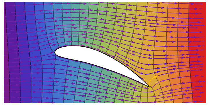
It can be compared with the potential flow around aerodynamic profile NACA9415 (close in parameters to the Zhukovsky profile). Flow without circulation (with circulation see here)
ClearAll[NACA9415];NACA9415[{m_,p_,t_},x_]:=Module[{},yc=Piecewise[{{m/p^2(2px-x^2),0<=x<p},{m/(1-p)^2((1-2p)+2px-x^2),p<=x<=1}}];yt=5t(0.2969Sqrt[x]-0.1260x-0.3516x^2+0.2843x^3-0.1015x^4);θ=ArcTan@Piecewise[{{(m*(2*p-2*x))/p^2,0<=x<p},{(m*(2*p-2*x))/(1-p)^2,p<=x<=1}}];{{x-ytSin[θ],yc+ytCos[θ]},{x+ytSin[θ],yc-ytCos[θ]}}];m=0.09;p=0.4;tk=0.15;pe=NACA9415[{m,p,tk},x];ParametricPlot[pe,{x,0,1},ImageSize->Large,Exclusions->None]ClearAll[myLoop];myLoop[n1_,n2_]:=Join[Table[{n,n+1},{n,n1,n2-1,1}],{{n2,n1}}]Needs["NDSolve`FEM`"];rt=RotationTransform[-π/9];(*angleofattack*)a=Table[pe,{x,0,1,0.01}];(*tableofcoordinatesaroundaerofoil*)p0={p,tk/2};(*pointinsideaerofoil*)x1=-2;x2=3;(*domaindimensions*)y1=-2;y2=2;(*domaindimensions*)coords=Join[{{x1,y1},{x2,y1},{x2,y2},{x1,y2}},rt@a[[All,2]],rt@Reverse[a[[All,1]]]];nn=Length@coords;bmesh=ToBoundaryMesh["Coordinates"->coords,"BoundaryElements"->{LineElement[myLoop[1,4]],LineElement[myLoop[5,nn]]},"RegionHoles"->{rt@p0}];mesh=ToElementMesh[bmesh,MaxCellMeasure->0.001];ClearAll[x,y,ϕ];sol=NDSolveValue[{D[ϕ[x,y],x,x]+D[ϕ[x,y],y,y]==NeumannValue[1,x==x1&&y1<=y<=y2]+NeumannValue[-1,x==x2&&y1<=y<=y2],DirichletCondition[ϕ[x,y]==0,x==0&&y==0]},ϕ,{x,y}∈mesh];ClearAll[vel];vel[x_,y_]:=Evaluate[Grad[sol[x,y],{x,y}]]st=StreamPlot[vel[x,y],{x,-.5,1.5},{y,-.5,.5},Epilog->{Line[coords[[5;;nn]]]},AspectRatio->Automatic,StreamPoints->Fine,StreamStyle->LightGray];dp=ContourPlot[sol[x,y],{x,-.5,1.5},{y,-.5,.5},ColorFunction->"Rainbow",Epilog->{Line[coords[[5;;nn]]]},AspectRatio->Automatic,Frame->False,Contours->20]bac=Show[dp,st]
Out[]=

Out[]=

Out[]=
Add animation
In[]:=
pX=ParametricNDSolveValue[{X'[t]==vel[X[t],Y[t]][[1]],Y'[t]==vel[X[t],Y[t]][[2]],X[0]==-1/2,Y[0]==y0},X,{t,0,5},{y0}];pY=ParametricNDSolveValue[{X'[t]==vel[X[t],Y[t]][[1]],Y'[t]==vel[X[t],Y[t]][[2]],X[0]==-1/2,Y[0]==y0},Y,{t,0,5},{y0}];pt=Table[Show[{dp,Graphics[Table[{LightGray,PointSize[.01],Point[Table[Evaluate[{pX[y0][t],pY[y0][t]}],{y0,-.5,.6,.0505}]]},{t,t0,t0+.5,.05}]]}],{t0,0,2.2,.1}];//QuietListAnimate[pt]
Finally, using the nonlinear FEM implemented in version 12, it is possible to calculate the viscous flow for profile NACA9415. Here we see a different picture, not similar to the potential flow.
CITE THIS NOTEBOOK
CITE THIS NOTEBOOK
Airfoil streamlines visualization with a Zhukovsky profile
by Alexander Trounev
Wolfram Community, STAFF PICKS, September 20, 2023
https://community.wolfram.com/groups/-/m/t/3016823
Based on MSE comment
by Alexander Trounev
Wolfram Community, STAFF PICKS, September 20, 2023
https://community.wolfram.com/groups/-/m/t/3016823
Based on MSE comment