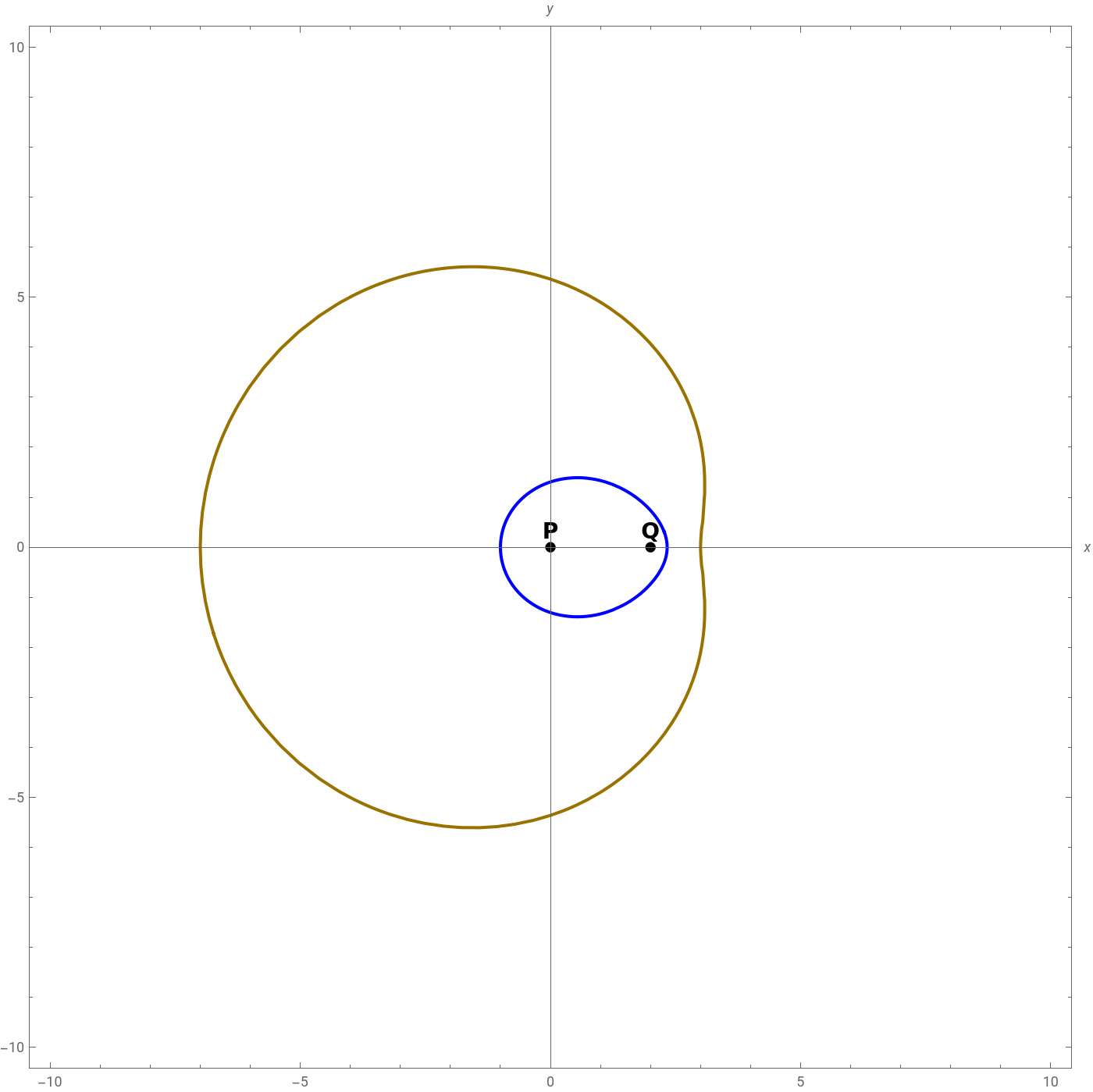
DifferentTypesDescartesOvals::usage="Let P and Q be two fixed points on the plane, and let d(P, S) and d(Q, S) the distances of these two points to a third variable point S. Being m and a two arbitrary real numbers, then, the cartesian oval is the geometric locus of the S(x, y) points that satisfy the condition that: d(P, S) ± m d(Q, S) == ± a. References: Personal.";
Animation: It is recommended for each sliding ruler to use the + and - signs to carefully observe each graph.
Suggested exercises (apart from the classic with which the notebook starts):
1) m = 1.0, c = 6.0, a = 8.0
2) m = 2.0, c = 2.0, a = 4.0
3) m = -1.0, c = 2.0, a = 1.5
1) m = 1.0, c = 6.0, a = 8.0
2) m = 2.0, c = 2.0, a = 4.0
3) m = -1.0, c = 2.0, a = 1.5
In[]:=
Manipulate[P={0,0};Q={c1,0};S={x,y};Show[{ContourPlot[Norm[P-S]+mNorm[Q-S]==a,{x,-w,w},{y,-w,w},ContourStyle->{Blue,Thick},MaxRecursion->3],ContourPlot[Norm[P-S]-mNorm[Q-S]==a,{x,-w,w},{y,-w,w},ContourStyle->{DarkYellow,Thick},MaxRecursion->3],ContourPlot[Norm[P-S]-mNorm[Q-S]==-a,{x,-w,w},{y,-w,w},ContourStyle->{DarkYellow,Thick},MaxRecursion->3],ContourPlot[Norm[P-S]+mNorm[Q-S]==-a,{x,-w,w},{y,-w,w},ContourStyle->{DarkYellow,Thick},MaxRecursion->3],Graphics[{Black,PointSize[0.01],Point[P],Text[Style["P",14,Bold],P,{0,-1.2}],Point[Q],Text[Style["Q",14,Bold],Q,{0,-1.2}]}]},AspectRatioAutomatic,AxesTrue,AxesOrigin{0,0},AxesLabel{x,y},PlotRangew,ImageSize700],Style["Descartes' Ovals",Bold,Large],{{w,10,"Value (w, PlotRange)"},5,20,0.5},Delimiter,{{c1,2,"Value (c, focus)"},-10,10,0.5},Delimiter,{{m,0.5,"Value (m)"},-10,10,0.5},Delimiter,{{a,2.5,"Value (a)"},1,10,0.5},ControlPlacementTop]
Out[]=