Wolfram Cloud Document

ABSTRACT (original article): We discuss slip bonds, catch bonds, and the tug-of-war mechanism using mathematical arguments. The aim is to explain the theoretical tool of molecular potential energy surfaces (PESs). For this, we propose simple 2-dimensional surface models to demonstrate how a molecule under an external force behaves. Examples are selectins. Catch bonds, in particular, are explained in more detail, and they are contrasted to slip bonds. We can support special two-dimensional molecular PESs for E- and L-selectin which allow the catch bond property. We demonstrate that Newton trajectories (NT) are powerful tools to describe these phenomena. NTs form the theoretical background of mechanochemistry. CITATION (original article): Quapp, W., & Bofill, J. M. (2024). Theory and Examples of Catch Bonds. In The Journal of Physical Chemistry B. American Chemical Society (ACS). DOI: https://doi.org/10.1021/acs.jpcb.4c00468

First we calculate the PES and Newton trajectories (NT) on it. Main direction (L+d) for dashed NT, comparison with (-1,1) for black NT. Blue is the corresponding singular NT, red the NT to direction (1,0)

First molecule LSelA108A + 2GSP6 : no.4 in Table of BB

ph0=0.58*Pi;d0=0.33;k0=266.0;D0=201.0;cc=0.0;ph1=0.97*Pi;sig=0.17*Pi;

PHI[L_]=2.0*ArcSin[L/5.6]De[ph_]=D0*Exp[-(ph-ph1)^2/(2.*sig^2)]+ccVphi[L_]=0.5*k0*(PHI[L]-ph0)^2Be[d_,ph_]=De[ph]*((1.0-Exp[-d/d0])^2-1.)pes[L_,d_,F_]=Vphi[L]+Be[d,PHI[L]]-(L+d)*F

conBarLSelA=ContourPlot[pes[L,d,0],{L,4.25,5.6},{d,-0.2,0.75},ContourShadingFalse,Contours50,PlotRange->All,PlotPoints53,ContourStyleThickness[0.00215],FrameLabel{"L","d"},AspectRatio1,FormatTypeTraditionalForm,FrameStyleFontSize16]

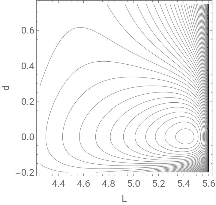
Derivations, here for traditional reasons, the second variable has no.3

p3[L_,d_]=D[pes[L,d,0],d];p1[L_,d_]=D[pes[L,d,0],L];p11[L_,d_]=D[p1[L,d],L];p33[L_,d_]=D[p3[L,d],d];p31[L_,d_]=D[p3[L,d],L];

For NTs the gradient has to be parallel to the search direction. In 2D we can plot the NT by the zero line of the interchanged coefficients of the gradient components NT1 is to (1,0), NT2 is to direction (-1,1)

NewT1=ContourPlot[p3[L,d],{L,4.25,5.6},{d,-0.2,0.15},ContourShading->False,PlotPoints->77,Contours->{0.0},ContourStyle->{Thickness[0.005],Red}]

NewT2=ContourPlot[p1[L,d]+p3[L,d],{L,4.25,5.6},{d,-0.22,0.75},ContourShading->False,PlotPoints->77,Contours->{0.0},ContourStyle->{Thickness[0.005],Black}]

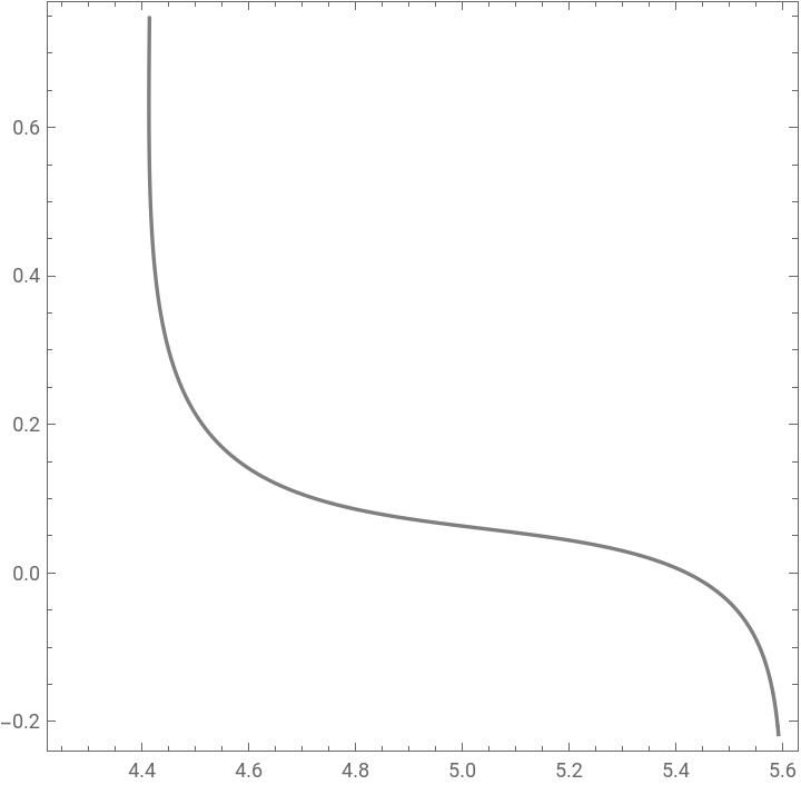
In 2D also the determinant of the Hessian matrix is simple

DetH[L_,d_]=Simplify[p11[L,d]*p33[L,d]-p31[L,d]*p31[L,d]];

We search for the line Det(H)=0 on the PES

deter1=ContourPlot[Evaluate[DetH[L,d],{L,4.25,5.6},{d,-0.2,0.75},ContourShadingFalse,PlotPoints40,Contours{0.0},ContourStyle{Thickness[0.0046],Green}]]

NT11 to direction (1,1), that one of main interest

NewT11=ContourPlot[p3[L,d]-1.0*p1[L,d],{L,4.25,5.6},{d,-0.2,0.75},ContourShading->False,PlotPoints->77,Contours->{0.0},ContourStyle->{Dashed,Thickness[0.0085]}]

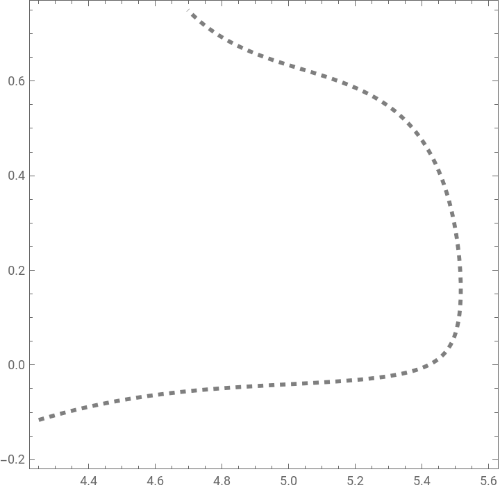
Next are data for the figures

spArr=Graphics[Arrow[{{4.537,0.65},{4.537,0.73}}]]textLSelA=Show[Graphics[{Text[Style["R"],{5.5540,-0.05}],Text[Style["TS"],{4.615,0.7}],Text[Style["LSelA108H"],{5.29,0.71}],Text[Style["+2GSP6"],{5.293,0.635}]},PlotRange{{L,1.5,5.5},{d,-.25,0.5}}]];BiLSelA=Show[conBarLSelA,NewT2,deter1,NewT1,NewTNT11,spArr,textLSelA,TextStyle->FontSize19]

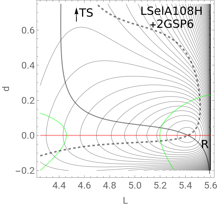
Export["BildLSelA108H.pdf",BiLSelA,ImageResolution400,ImageSizeAutomatic]

Next example
LSelN138G + PSGL1: no.2 in BB tabelle

ph0=0.58*Pi;d0=0.29;k0=220.0;D0=210.0;cc=0.0;ph1=Pi;sig=0.12*Pi;

PHI[L_]=2.0*ArcSin[L/5.6]De[ph_]=D0*Exp[-(ph-ph1)^2/(2.*sig^2)]+ccVphi[L_]=0.5*k0*(PHI[L]-ph0)^2Be[d_,ph_]=De[ph]*((1.0-Exp[-d/d0])^2-1.)pes[L_,d_,F_]=Vphi[L]+Be[d,PHI[L]]-(L+d)*F

The singular NT through the VRI point must be determined by hand, it means one has to probe the coefficients for the searched intersection of the two branches of the NT , drawn in blue

L-selectin + 2GSP6 no.3 in BB Table

L-selectin + PSGL1 vorher falsch k0=299.0 Haupteil !!!
No 1 in Tabelle in PNAS ist auch gleich !!!!! D.h. L-selectin alles wie vorher

Phi(L) indirekt gegeben !! W=2.8

Intermediate

Min R

Control of kind of stat points

Vorher NewT1

VRI point ~ (4.64, 0.1675)

Calculation of the catch bond barriers

Here we obtain a nice catch bond behavior

CITE THIS NOTEBOOK

Theory and examples of catch bonds
by Wolfgang Quapp
Wolfram Community, STAFF PICKS, May 1, 2024
https://community.wolfram.com/groups/-/m/t/3167380