Introduction
Introduction
In the theory of automata ϵ - non deterministic finite automata (ϵ-NFA) are essential to be able to construct automata easily, specially if in the regular expression there are choices (like a|b for example). an ϵ-NFA is basically the same as an NFA, but with some transitions labelled ϵ (empty symbol), which allows the NFA to move to another state without consuming or processing a symbol from the alphabet.
Here I show how to build ϵ-NFA using Mathematica. I assume that you already have some knowledge on Automata Theory. I have already posted about deterministic automata and non deterministic automata.
Formal definition of a ϵ-NFA
Formal definition of a ϵ-NFA
Formally it is define as an NFA , where,
E(Q,Σ,δ,,F)
q
0
◼
Q
◼
Σ
◼
δ:QΣ⋃{ϵ}
Q
2
ϵ
Σ⋃{ϵ}
◼
A starting state ∈Q
q
0
◼
A set of final states
F⊆Q
the empty symbol ϵ is not part of the alphabet but it is included in the mapping. This allows for moving simultaneously around different states and in some ways, process string in parallel. It will become clear in the examples.
Building some Mathematica code for ϵ-NFA
Building some Mathematica code for ϵ-NFA
Consider the following example,
ShowGraphFA[{01,03,12,21,34,45,53},{0,1,2,3,4,5},{0},{1,3},{"ϵ","ϵ","a","a","a","a","a"}]
Out[]=
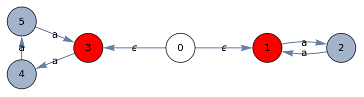
This automata accepts (Example taken from Sipser’s book). Notice how from the starting node 0, you can go either to node 1, or to node 3 without using any symbol. When the automata receives a string, it computes both sides in parallel, one side determines if the string has an even number of “a” and the other side check “a” in multiples of 3.
{|nis even or divisible by3}
n
a
The transition table,
FATable[δ,{0,1,2,3,4,5},{ϵ,"a"}]
Out[]=
Q\Σ | ϵ | a |
0 | {1,3} | - |
1 | - | {2} |
2 | - | {1} |
3 | - | {4} |
4 | - | {5} |
5 | - | {3} |
Codes for creating the graph and transition table are given at the end.
In Mathematica, we use Associations to build the transition function,
In[]:=
δ=Association[{0,ϵ}{1,3},{1,"a"}{2},{2,"a"}{1},{3,"a"}{4},{4,"a"}{5},{5,"a"}{3}];
Notice how a Key takes a state and a symbol (“a” or “b”) or the empty symbol ϵ, and return a Value that is a list, with one or more states, that is, {state,”symbol”} {states}, just as mathematically define above.
The first thing we have to create is a function that calculates what is called the ϵ-Closure of a state. Informally it is defined as all the states reachable from a state using ϵ transitions. To do this, we have to follow all the paths that can be travelled using only ϵ transitions. For this we can use NestWhileList, that operates over δ.
But first since δ returns a list of states, then we have to evaluate each one of them, we can use a pure function for this. Here I show you how, and evaluate for state 0,
Table[δ[{#1[[i]],ϵ}]/._Missing{},{i,Length[#1]}]&[{0}]
Out[]=
{{1,3}}
Notice how we get all the ϵ transitions of state 0 (highlighted in red). Now we can use this in a NestWhileList,
NestWhileList[Union@@Table[δ[{#1[[i]],ϵ}]/._Missing{},{i,Length[#1]}]&,{0},#≠{}&]
Out[]=
{{0},{1,3},{}}
This evaluates all the paths from state 0 (in red). Notice also that the stopping condition in the NestWhileList, is an empty set (we replace Missing Keys with empty set {}), we can remove that last item on the list. Now we can build a function that puts everything together,
In[]:=
Closure[δ_,state_List]:=Union[Map[Flatten[Most[NestWhileList[Union@@Table[δ[{#1[[i]],ϵ}]/._Missing{},{i,Length[#1]}]&,{#},#≠{}&]/._Missing{}]]&,state]//Flatten]
So, the ϵ-Closure of 0, is then given by,
Closure[δ,{0}]
Out[]=
{0,1,3}
Now we are ready to create our extended function that computes an entire string. I will not give mathematical details, but it follows the definition that can be found in Hopcroft & Ullman’s book (see references). Informally, it calculates all the paths that can be follow given a symbol, and then it also follow further ϵ transitions (applying the ϵ-Closure function we just made),
δ
In[]:=
DeltaHatEpsilon[δ_,q0_List,string_]:=FoldList[Closure[δ,Union@@Table[δ[{#1[[i]],#2}]/._MissingNothing,{i,Length[#1]}]]&,Closure[δ,q0],Characters[string]]
Now we can test our function with string “aaa”. The starting state is 0 and the final states {1,3}
DeltaHatEpsilon[δ,{0},"aaa"]
Out[]=
{{0,1,3},{2,4},{1,5},{2,3}}
The last state list of the result, contains state 3, which is a final state, therefore the string is accepted (has 3 “a” which is a multiple of 3). Notice how each element of the list, corresponds to each symbol in the string evaluated (from left to right). Now let’s try “aaaa”,
DeltaHatEpsilon[δ,{0},"aaaa"]
Out[]=
{{0,1,3},{2,4},{1,5},{2,3},{1,4}}
The last state list of the result, contains state 1, then the string is accepted ( has even number of “a”).
How about “aaaaa”,
DeltaHatEpsilon[δ,{0},"aaaaa"]
Out[]=
{{0,1,3},{2,4},{1,5},{2,3},{1,4},{2,5}}
Notice that the last list of the result, does not contain a final state, therefore the string is not accepted.
More Examples
More Examples
Taken from Sipser’s book,
ShowGraphFA[{01,04,12,23,45,46,57,67,70},{0,1,2,3,4,5,6,7},{0},{3},{"ϵ","ϵ","a","c","ϵ","ϵ","a","b","ϵ"}]
Out[]=
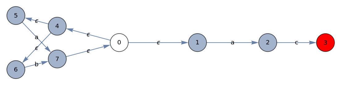
This automata can write expressions that can multiple combinations of a or b, but end in ac. This automata produces the regular expression (a|b)*ac. Nodes 4-7 result in the (a|b)* and 1-3 with the ending ac. Notice how from node 4-7 resolves the a|b strings .
The transition table,
FATable[δ,{0,1,2,3,4,5,6,7},{ϵ,"a","b","c"}]
Out[]=
Q\Σ | ϵ | a | b | c |
0 | {1,4} | - | - | - |
1 | - | {2} | - | - |
2 | - | - | - | {3} |
3 | - | - | - | - |
4 | {5,6} | - | - | - |
5 | - | {7} | - | - |
6 | - | - | {7} | - |
7 | {0} | - | - | - |
Our δ function,
In[]:=
δ=Association[{0,ϵ}{1,4},{1,"a"}{2},{2,"c"}{3},{4,ϵ}{5,6},{5,"a"}{7},{6,"b"}{7},{7,ϵ}{0}];
COmpute the string “ababac”
DeltaHatEpsilon[δ,{0},"ababac"]
Out[]=
{{0,1,4,5,6},{0,1,2,4,5,6,7},{0,1,4,5,6,7},{0,1,2,4,5,6,7},{0,1,4,5,6,7},{0,1,2,4,5,6,7},{3}}
Which is accepted (final list contains state 3), and string “abababa”
The final list does not contain state 3, so this string is not valid.
Extra code (graph and table)
Extra code (graph and table)
I will not give details on how to build these functions. I think they are easy to follow,
References
References
◼
Hopcroft and Ullman, Introduction to Automata Theory, Languages and Computation, Addison Wesley.
◼
Michael Sipser, Introduction to theTheory of Computation. PWS Publishing Company, 2006.