ABSTRACT (original article): In the present paper, we present the solution of four problems drawn from the chemical and biochemical engineering field of study. These problems illustrate various important aspects of nonlinear dynamics such as limit cycles, quasi-periodic and chaotic behaviors, time series and phase portraits, power spectra, the time-delay reconstruction diagrams, Hopf bifurcation, bifurcation diagrams, steady state multiplicity… Among a large number of examples, we have selected the following case studies because they illustrate the basic nonlinear dynamics concepts listed previously: (i) The glycolytic oscillator model, first suggested by Sel’kov in 1968 in order to elucidate the mechanism that living cells use to obtain energy from sugar breakdown; (ii) The Oregonator model derived by Field, Körös, and Noyes in the early 1970s, which elucidates the famous oscillatory behavior observed in the Belousov–Zhabotinsky reaction; (iii) The steady state multiplicity in a biochemical reactor for both the Monod and substrate inhibition kinetics; and (iv) The three-variable autocatalator, first proposed by Peng, Scott, and Showalter in 1990. Finally, we conclude this paper by sharing our experience teaching this subject to graduate students at King Fahd University of Petroleum & Minerals (KFUPM). CITATION (original article): Binous H., Bellagi A., Introducing nonlinear dynamics to chemical and biochemical engineering graduate students using MATHEMATICA©, Computer Applications in Engineering Education, 2019; 27: 217–235. https://doi.org/10.1002/cae.22070
In the study of nonlinear dynamics, it is useful to first introduce students to simple systems that exhibit periodic behavior as a consequence of a Hopf bifurcation. For instance, the glycolytic oscillator model has this feature. This model was first suggested by Sel’kov in 1968 in order to elucidate the mechanism that living cells use to obtain energy from sugar breakdown. This two-dimensional nonlinear and autonomous system, is given by
=(x,y)=-x+ay+y
=(x,y)=b-ay-y
x
f
1
2
x
y
f
2
2
x
These equations describe the autocatalytic reaction of two intermediate species and in an isothermal batch reactor, when the system is far from equilibrium [1]. In this context, the steady state referred to below is a pseudo steady state, and is applicable when the precursor reactant is slowly varying with time.
x
y
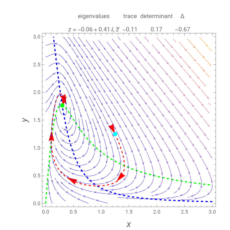
The unique steady state is given by =b and =b/(a+). This steady state is at the position of the green dot in the phase portrait diagram. It appears as the intersection of the dotted blue and green curves, which are the level curves given by (x,y)=0 and (x,y)=0. The stability of steady state to small disturbances can be assessed by determining the eigenvalues of the Jacobian . A Hopf bifurcation occurs when a complex conjugate pair of eigenvalues crosses the imaginary axis.
x
S
y
S
2
b
f
1
f
2
J=
∂ f 1 | ∂ f 1 |
∂ f 2 | ∂ f 2 |
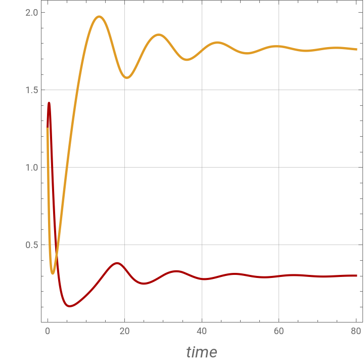
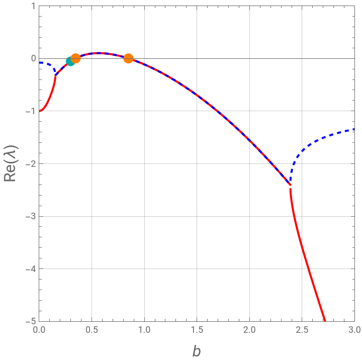
We show the phase portrait with the vector field of directions around the critical point . In addition, the eigenvalues of , the trace , the determinant , and -4J are computed. The time series are also plotted in a separate diagram (the blue and red curves correspond to and , respectively. Finally, the real and imaginary parts of the two eigenvalues and are plotted (in blue and red, respectively) versus for several values of the parameter .
(,)
x
S
y
S
J
tr(J)
J
2
Δ=tr(J))
x(t)
y(t)
λ
1
λ
2
b
a
To observe a Hopf bifurcation, you can set and vary . As shown in this notebook, there are two Hopf bifurcation points. Indeed, for , the steady state is a stable focus; for , the trajectory is attracted to a stable periodic solution (called a limit cycle); and finally for , the steady state is again a stable focus.
For, the two Hopf bifurcation points are obtained at and .
a=0.08
b
b=0.3
b=0.5
b=1.0
For
a=0.08
b=0.34641
b=0.848528
Finally, for the last calculation (obtained for larger values of , for instance, ), the Hopf bifurcation disappears and there are only transitions from a stable node to a stable focus and then back to stable node.
a
a=0.65
Two-dimensional nonlinear and autonomous system that describes the mechanism of glycolysis:
f1[x_,y_]:=-x+a*y+x^2y;f2[x_,y_]:=b-a*y-x^2*y;
Steady-states:
solSS=Flatten@NSolve[{-x+a*y+x^2y0,b-a*y-x^2*y0},{x,y}];
Jacobian matrix:
m1=Outer[D,{f1[x,y],f2[x,y]},{x,y}];
m=m1/.solSS;
Eigenvalues of Jacobian matrix:
Eig=Chop@N@Eigenvalues[m];
Initial condition:
x0={1.25,1.25};
a and b values:
a=0.08;b=0.30;
Solution of the dynamical system:
sol=NDSolve[{x'[t]-x[t]+a*y[t]+x[t]^2y[t],y'[t]b-a*y[t]-x[t]^2*y[t],x[0]x0[[1]],y[0]x0[[2]]},{x,y},{t,0,500},Method"StiffnessSwitching"];
Time series plot indicate damped oscillations - the eigenvalues are complex conjugates with negative real parts:
p1=Plot[Evaluate[{x[t],y[t]}/.sol],{t,0,80},PlotRangeAll,PlotStyle{Darker@Red,Thickness[0.007]},PlotPoints1000,AspectRatio1,FrameTrue,GridLinesAutomatic,FrameLabel{Style["time",16,Italic],Style["",16,Italic]},PlotPoints100,PlotLegends{Style["x",16,Italic],Style["y",16,Italic]}]
Out[]=


Eigenvalues:
zz=Chop@N@Eigenvalues[m];
Parametric plot:
p1=ParametricPlot[Evaluate[{x[t],y[t]}/.sol],{t,0,50},PlotRangeAll,PlotStyle{Darker@Red,Dashed,Thickness[0.007]},PlotPoints1000];xx=First[Cases[p1,x_LineFirst@x,Infinity]];
In[]:=
ShowContourPlot{-x+a*y+x^2y==0,b-a*y-x^2*y0},{x,0,3},{y,0,3},PlotLabelGridTranspose@"eigenvalues",IfIm[First@zz]0,NumberForm[zz,{4,2}],RowStyle["z",Italic]," = ",NumberForm[First@zz,{4,2}],", ",,{"trace",NumberForm[Chop@N@Tr[m],{4,2}]},{"determinant",NumberForm[Chop@N@Det[m],{4,2}]},{"Δ",NumberForm[Chop@N@Tr[m]^2-4Det[m],{4,2}]},ItemSize({#,Automatic}&/@{10,4,4,4}),FrameLabel{Style["x",16,Italic],Style["y",16,Italic]},PlotPoints100,ContourStyle{{Green,Thick,Dashed,Opacity[0.99]},{Blue,Dashed,Thick,Opacity[0.99]}},Epilog{Green,PointSize[0.025],Point[{x,y}/.solSS],Cyan,Point[x0]},Graphics[{Red,Arrowheads[Table[0.06,{6}]],Dashed,Thickness[0.005],Arrow[Line[Partition[xx,Floor[Length[xx/10]]][[;;;;100]]]]}],StreamPlot[{-x+a*y+x^2y,b-a*y-x^2*y},{x,0,3},{y,0,3},StreamStyleDirective[Opacity[0.5]],StreamPoints50],ImageSize400{1,1},ImagePadding{{50,Automatic},{Automatic,Automatic}}
Style["z",Italic]
Out[]=
Let us determine the critical values of b when a=0.08
-- at these values both eigenvalues are purely imaginary shown below by the orange dots --
cyan dots are for b=0.3
-- at these values both eigenvalues are purely imaginary shown below by the orange dots --
cyan dots are for b=0.3
b1c=0.3464101615137754;b2c=0.848528137423857;
Two-dimensional nonlinear and autonomous system that describes the mechanism of glycolysis:
f1b1[x_,y_]:=-x+a*y+x^2y;f2b1[x_,y_]:=b1-a*y-x^2*y;
Steady-states:
solSSb1=Flatten@Quiet@Solve[{-x+a*y+x^2y0,b1-a*y-x^2*y0},{x,y}];
Jacobian matrix:
m2=Outer[D,{f1b1[x,y],f2b1[x,y]},{x,y}]/.solSSb1;
Eigenvalues of Jacobian matrix:
{λ1,λ2}=Eigenvalues[m2];
Show[Plot[{Re[λ1],Re[λ2]},{b1,0,3},PlotStyle{{Red,Thick},{Blue,Dashed,Thick}},FrameTrue,FrameLabel{Style["b",Italic,16],Style["Re(λ)",16]},PlotRange{{0,3},{-5,1}},GridLinesAutomatic,AspectRatio1],Graphics[{Darker@Cyan,PointSize[0.03],Point[{b,Re[Eig[[1]]]}],Point[{b,Re[Eig[[2]]]}],Orange,PointSize[0.032],Point[{b1c,0}],Point[{b2c,0}]},ImagePadding{{40,Automatic},{40,Automatic}}],ImageSize.9×400{1,1}]
Show[Plot[{Im[λ1],Im[λ2]},{b1,0,3},PlotStyle{{Red,Thick},{Blue,Dashed,Thick}},FrameTrue,FrameLabel{Style["b",Italic,16],Style["Im(λ)",16]},PlotRange{{0,3},{-3,3}},GridLinesAutomatic,AspectRatio1],Graphics[{Darker@Cyan,PointSize[0.03],Point[{b,Im[Eig[[1]]]}],Point[{b,Im[Eig[[2]]]}]},ImagePadding{{40,Automatic},{40,Automatic}}],ImageSize.9×400{1,1}]
Out[]=
Determination of the critical values of b when a = 0.08
Color function for the contour plot given below:
Two-dimensional nonlinear and autonomous system that describes the mechanism of glycolysis:
Steady states:
Jacobian matrix:
Critical values of b when a=0.08:
We consider only positive b:
In[]:=
(*b=1.0 and a=0.08*)
In[]:=
(*b=0.4 and a=0.08*)
In[]:=
(*a=0.65 and b=0.05;*)
Acknowledgement
Acknowledgement
Some of the coding was written in collaboration with Prof. B. G. Higgins.
CITE THIS NOTEBOOK
CITE THIS NOTEBOOK
The glycolytic oscillator mechanism
by Housam Binous and Ahmed Bellagi
Wolfram Community, STAFF PICKS, April 8, 2024
https://community.wolfram.com/groups/-/m/t/3154806
by Housam Binous and Ahmed Bellagi
Wolfram Community, STAFF PICKS, April 8, 2024
https://community.wolfram.com/groups/-/m/t/3154806