Analysis of the Change in Phillips Curve After the Coronavirus Pandemic Using Linear Regression by Seojin (Heidi) Yoon
I recently encountered an article about the dangers of a ‘disaster scenario’ of the coronavirus pandemic, which is the occurrence of stagflation. Hence, I attempted to predict the possibility of stagflation due to COVID-19 in Korea.
Introduction
Introduction
COVID-19 and the Economic Impacts
COVID-19 and the Economic Impacts
COVID-19 put many unemployed, due to the reduction in hiring rate, and as many companies have been put out of business. Following the outbreak, global stock markets crashed, and the fear of a lockdown caused panic buying, which led to supply shortage of essential items. Industries related to leisure like travel industries were most severely damaged, and technology industries were hindered due to the delay in shipments. The COVID-19 pandemic is considered to be one of the largest global recession in history.
Phillips Curve
Phillips Curve
Phillips curve is an economic model that represents the relationship between inflation and unemployment. According to the model, inflation and unemployment follow an inversely proportional relationship, because inflation occurs as a result of economic development, and with economic growth comes more jobs.
Stagflation
Stagflation
The Phillips curve generally makes sense regardless of a country’s economic state. However, this was shown invalid in the early 1970s, when stagflation occurred. Stagflation is the undesirable occurrence of both high inflation rate and unemployment rate. Stagflation may occur when money supply is expanded (one of the reasons being the printing of currency) whereas the supply is limited which may be due to a national crisis such as the war. Both seemed likely in this situation of a global pandemic, and therefore, I decided to investigate the potential risk of stagflation by comparing inflation and unemployment data after the corona outbreak to the predicted Phillips curve model before the outbreak.
Goal
Goal
The goal of this investigation is to determine the effects of COVID-19 on the Korean economy, using the gradient descent algorithm for regression. The inversely related curve of monthly inflation and unemployment rate data of about 10 years would be approximated with regression, and then data from after the coronavirus outbreak would be compared to the curve.
Inflation and Unemployment Data
Inflation and Unemployment Data
Getting Data
Getting Data
Monthly inflation and unemployment rates in South Korea between January 2010 to May 2020 were downloaded from the following links:
http://kosis.kr/statHtml/statHtml.do?orgId=101&tblId=DT_ 1J17042&checkFlag=N (Inflation rate)
http://kosis.kr/statHtml/statHtml.do?orgId=101&tblId=DT_1DA7004S (Unemployment rate)
http://kosis.kr/statHtml/statHtml.do?orgId=101&tblId=DT_ 1J17042&checkFlag=N (Inflation rate)
http://kosis.kr/statHtml/statHtml.do?orgId=101&tblId=DT_1DA7004S (Unemployment rate)
Peak Analysis
Peak Analysis
When the two sets of data (inflation and unemployment rate) were graphed, they roughly appeared to share similar increasing and decreasing trends.
Out[]=


However, when inflation and unemployment data matched directly to one another according to the change in time was processed, almost no inverse correlation existed between the two. This was because with increase in inflation follows the decrease in unemployment afterwards, so inflation rate and unemployment rate will not show an inverse relationship when graphed simultaneously. However, merely shifting the two graphs did not improve correlation, which may be because the time it takes for unemployment to occur as a result of inflation does not stay constant.
In[]:=
Table[ListLinePlot[{Drop[Table[datatest[[n]][[1]],{n,Length[datatest]}],-t],Drop[Table[datatest[[n]][[2]],{n,Length[datatest]}],t]},PlotLegends{"Inflation","Unemployment"},PlotLabel"Shift inflation by "<>ToString@t<>" months to the right"],{t,8}]
Out[]=
,
,
,
,
,
,
,
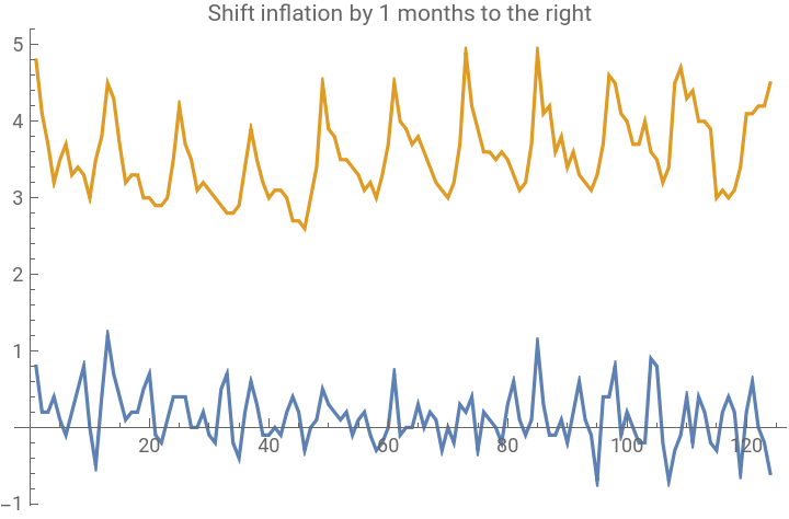
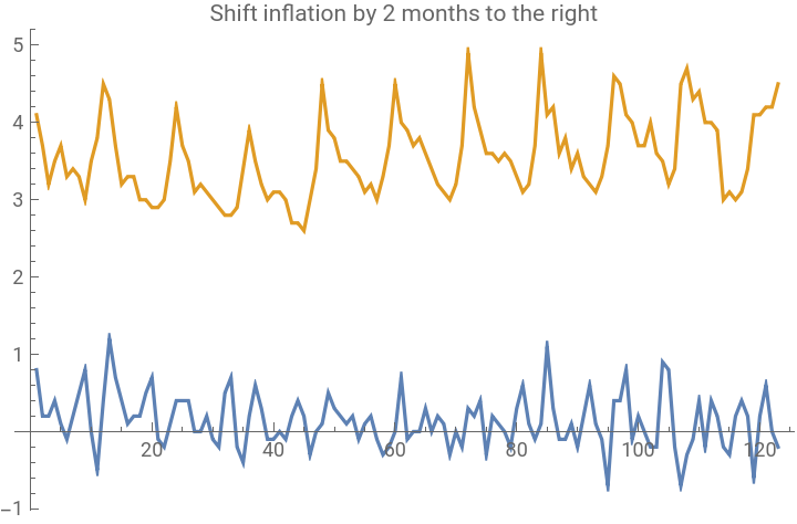
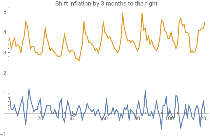
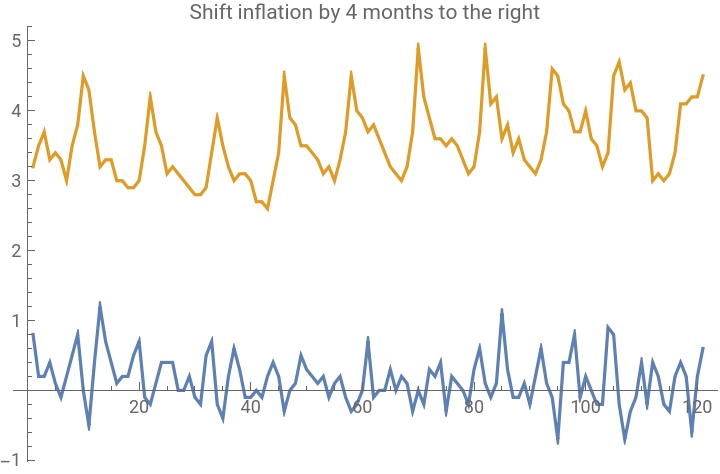
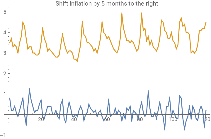
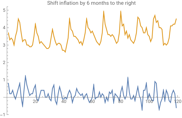
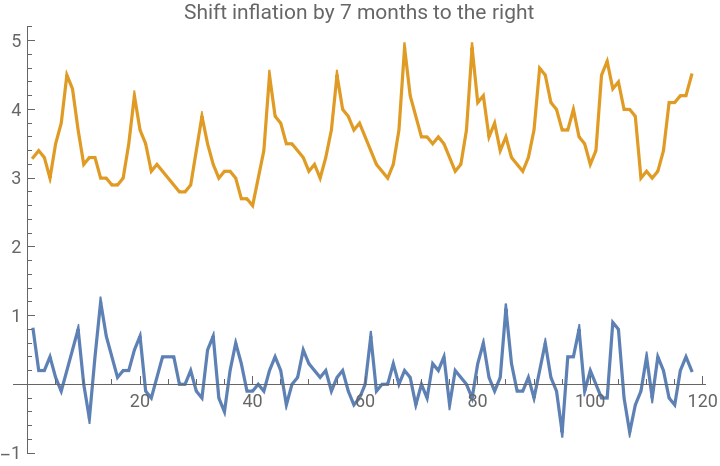
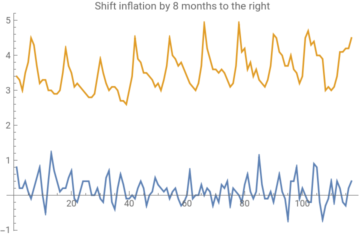
Therefore, data was manipulated in python by aligning unemployment and inflation data peak-by-peak (the max peak of one will be matched with the min peak of the other), and interpolating data in between.
Link to the python code: https://github.com/syoon2021/PhillipsCurve
Link to the python code: https://github.com/syoon2021/PhillipsCurve
To begin with, peaks were identified by collecting points in which the change in sign of slope occurred before and after the point. Then, peaks under the threshold for being a true peak were eliminated. In this process occurred two peaks of same concavity, so these were merged. Once all peaks of unemployment and inflation were identified, it was assumed that the two follow an inverse relationship, so the positive peak of one was matched to the negative peak of the other. The graphs were then flattened smoothly by interpolating equal number of data points in between the matched peaks.
Opening Interpolated Data
Opening Interpolated Data
The resultant data was brought up in Wolfram Alpha. The function ReadData creates a list of lists containing the features. Given a data file, all numerical values are separated by the comma and line, and each elements in a feature is combined as a list by grouping the list with numFeatures (number of features). All elements are converted into numbers from string using ToExpression.
There are two features for this investigation--inflation rate and unemployment rate--so the interpolated data from python was saved as a list of lists separated by every two elements.
A demonstration on why elements are split into lists by the number of features:
The data received from python was in the form of a pair of the two features, with each pair separated with a line. As inflation and unemployment data alternates, they were grouped into two to create lists of pairs.
Data Normalization
Data Normalization
There was one case to look out for. If there is only one element in a data, since the standard deviation is zero, the z score will be dividing by zero. This gives an undefined value, so if there is only one element in a data, or the standard deviation is zero, the element is returned as it is. Otherwise, the difference between data values and their mean is divided by the standard deviation. The function repeat is used to create a list of mean and standard deviation of the same length as the data, so that normalization can occur simultaneously as a list.
An approximation of the Phillips curve using higher polynomials will be done using regression, which means that the range of data will increase by a greater amount according to the power. In order to ensure that the gradient descent algorithm converge in a feasible time, data normalization will later be applied to each degree.
Demonstration on why to normalize within each degree (why range of data increase according to power):
Gradient Descent
Gradient Descent
Why gradient descent?
Why gradient descent?
I decided to use the gradient descent algorithm to analyze the unemployment and inflation relationship for higher degree polynomial approximation. I initially attempted to use the Nonlinearmodelfit function on Wolfram Alpha, but noticed that using the function didn’t ensure convergence for higher degree polynomial approximation, as it required convergence within 100 iterations. I recently learned about the gradient descent algorithm that is often used in machine learning, so I thought it would be interesting to try it using the Wolfram language.
What is the gradient descent method?
What is the gradient descent method?
Learning Rate
Learning Rate
Cost Function
Cost Function
Gradient Descent with Cost Function
Gradient Descent with Cost Function
Gradient Descent for Higher Degree Polynomials
Gradient Descent for Higher Degree Polynomials
Vectorization
Vectorization
The function GradientDescent calculates the gradient for each iteration with c representing the error. When later inserted in a loop, the algorithm would calculate the error and gradient for each of the iterations.
Regularization
Regularization
Regression
Regression
Regression with Higher Polynomials
Regression with Higher Polynomials
For regression with higher polynomials, a list of x values of different power is first made, to treat each of the x^i values as different features. Hence, with the function MapFeatures, x is powered, with a for loop that inserts increasing values of i. The x values are normalized for each loop of increasing i, to ensure that data values are normalized within each degree. For each degree, the mean and standard deviation are saved into the lists muFeatures and sFeatures for future use (function MapValue).
Initially, I tried regression with Taylor approximation, but discovered that adding a 1/x term produced a better approximation. Hence, i in x^i will start from -1 to d.
Applying Gradient Descent
Applying Gradient Descent
Now gradient descent algorithm can be applied. To begin with, all theta values are arbitrarily set as 0:
The last 20 data points for inflation and unemployment rate were approximately data points after the corona virus pandemic occurred, so they were excluded from the training data. Alpha = 0.01, lambda = 0.03, d = 10 seemed to give the best approximation.
Using the mean and standard deviation values of each degree saved from MapFeatures, the function MapValue expands, then normalizes all data values from degree of -1 to d.
The function MapValue was applied for graphing. Since MapValue creates lists of powered data values, the output was multiplied to the coefficients (each theta values) to take form of a function.
A simple demonstration on what the MapValue function does (excluding normalization):
Therefore, multiplying the results of MapValue to the list of theta values produces the desired polynomial function.
The best fit Phillips Curve obtained from the training data (p2), the training data excluding the last 20 data points (p1), and the test data of the last 20 data points (p3) were graphed together.
The test data seemed to lie above the original Phillips Curve model, but whether it really does can be determined by comparing with other time periods. The inflation and unemployment data were separated by every 20 data points, with the last 20 being data from after the corona virus pandemic. For each 20, the mean of squared error was calculated.
Conclusion
Conclusion
In general, all error values are pretty low, which indicates that the curve is a good approximation of the data. The last 20 data from after the coronavirus outbreak has the mean error of 0.0254506, which is even less than the average of all errors, 0.0977708. Hence, the error between the test data and the initial Phillips Curve model is reasonable enough to conclude that there are no clues of stagflation as of now. I can continue to monitor the risk of stagflation, because the algorithm is made so that the addition of new data is possible without any changes.
Limitations
Limitations
One limitation of this investigation is that the Phillips curve is not applicable for long term evaluation. Since inflation and unemployment data of about the span of 10 years was used for regression, an inversely proportional relationship between the two may not apply. Another limitation is that the raw data may have been overly manipulated, as the peaks were matched and data points were interpolated, carrying the assumption that inflation and unemployment was inversely related. Moreover, evaluating the effects of COVID-19 before the situation is over may provide only a limited insight, because the the effects of both before and after COVID-19 cannot be compared.
Extensions
Extensions
The traditional Phillips Curve takes form of an inverse relationship, but this was shown invalid for analysis of the long run, so new models for long term evaluation were made. Since this investigation shows that the analysis of relationship between unemployment and inflation can be done with regression, I can extend this to more relevant models.
Works Cited
Works Cited
Business, Paul R. La Monica, CNN. “The Coronavirus Economic ‘disaster’ Scenario: Stagflation.” CNN, https://www.cnn.com/2020/03/10/investing/stagflation-economy-coronavirus/index.html.
Chakrabarty, Navoneel. “Implementation of Multi-Variate Linear Regression in Python Using Gradient Descent Optimization….” Medium, 25 Mar. 2019, https://towardsdatascience.com/implementation-of-multi-variate-linear-regression-in-python-using-gradient-descent-optimization-b02f386425b9.
“Economic Impact of the COVID-19 Pandemic.” Wikipedia, 9 Aug. 2020. Wikipedia, https://en.wikipedia.org/w/index.php?title=Economic_impact _of _the _COVID-19_pandemic&oldid=971964046.
Gradient Descent and Stochastic Gradient Descent - Mlxtend. http://rasbt.github.io/mlxtend/user_guide/general_concepts/gradient-optimization/.
Gradient Descent Derivation · Chris McCormick. https://mccormickml.com/2014/03/04/gradient-descent-derivation/.
Gupta, Prashant. “Regularization in Machine Learning.” Medium, 16 Nov. 2017, https://towardsdatascience.com/regularization-in-machine-learning-76441ddcf99a.
KOSIS. http://kosis.kr/statHtml/statHtml.do?orgId=101&tblId=DT_ 1J17042&checkFlag=N.
KOSIS. http://kosis.kr/statHtml/statHtml.do?orgId=101&tblId=DT_ 1DA7004S.
Liu, Yang. “Vectorization Implementation in Machine Learning.” Medium, 23 Oct. 2018, https://towardsdatascience.com/vectorization-implementation-in-machine-learning-ca652920c55d.
Mainkar, Sagar. “Gradient Descent in Python.” Medium, 28 Aug. 2018, https://towardsdatascience.com/gradient-descent-in-python-a0d07285742f.
Menon, Adarsh. “Linear Regression Using Gradient Descent.” Medium, 19 Sept. 2018, https://towardsdatascience.com/linear-regression-using-gradient-descent-97a6c8700931.
Palumbo, Lora Jones, Daniele, and David Brown. “Coronavirus: A Visual Guide to the Economic Impact.” BBC News, 30 June 2020. www.bbc.com, https://www.bbc.com/news/business-51706225.
Pandey, Parul. “Understanding the Mathematics behind Gradient Descent.” Medium, 17 Jan. 2020, https://towardsdatascience.com/understanding-the-mathematics-behind-gradient-descent-dde5dc9be06e.
“Regularization (Mathematics).” Wikipedia, 1 Aug. 2020. Wikipedia, https://en.wikipedia.org/w/index.php?title=Regularization_(mathematics)&oldid=970651838.
Yıldırım, Soner. “Time Series Analysis: Resampling, Shifting and Rolling.” Medium, 15 Apr. 2020, https://towardsdatascience.com/time-series-analysis-resampling-shifting-and-rolling-f5664ddef77e.
Image Citations
Image Citations
[1] Liu, Yang. “Vectorization Implementation in Machine Learning.” Medium, 23 Oct. 2018, https://towardsdatascience.com/vectorization-implementation-in-machine-learning-ca652920c55d.
[2] “Regularization (Mathematics).” Wikipedia, 1 Aug. 2020. Wikipedia, https://en.wikipedia.org/w/index.php?title=Regularization_(mathematics)&oldid=970651838.
[2] “Regularization (Mathematics).” Wikipedia, 1 Aug. 2020. Wikipedia, https://en.wikipedia.org/w/index.php?title=Regularization_(mathematics)&oldid=970651838.