Introduction
In the previous bi-radial matrix article a space time network was introduced by extending a geometric analogy to gravitation. This forms two sets of equi-spaced radial lines each of these
corresponding to a spherical mass of uniform density; this giving rise to a geometric analogy of two interacting gravitational fields. One of the basic properties of this matrix is that it is “invariant
under spatial transformation”. The resulting quantized interference pattern yielded a network of intersection nodes. Applying two connection algorithms a prototypical model of magnetic
attraction and repulsion lines were formed. Further analysis revealed inverse square relations over distance embedded in the structure.
With respect to quantum reconstruction extending to the macroscopic realm we are deriving a quantum geometry which is scalable from the microscopic to the macroscopic realm.
To derive this from a set of fundamental principles. This includes the fundamental relation between space and time, i.e. motion and reevaluating the separate definitions of space and time.
From these and other basic principles and the many ways these can be combined arrive at descriptions of more complex phenomenon. The basic properties of time is a subject of serious debate
in physics. That space in time are closely interrelated in the form of a space time continuum is integral to general relativity.
As in the previous article there are three main sections of code. Section 1 is presented here and the other two are at the end of this article.
Biradial Manipulate
Biradial Manipulate
Begin Package
Begin Package
BeginPackage["BiRadialMatrix`", {"GeneralUtilities`"}]
Needs[# <> "`", FileNameJoin[DirectoryName[$InputFileName], # <> ".wl" ]]& /@ { "BiradialPlot"}
Usage Statements
Usage Statements
SetUsage[BiradialManipulate, "BiradialManipulate[]"]
Begin Private
Begin Private
Begin["`Private`"] (* Begin Private Context *)
Manipulate
Manipulate
BiradialManipulate[] := DynamicModule[ pha = 0, phb = 0, phaseSync = False, phaseInverse = False, showLabels = False, mirrorRayNumbering = False , Manipulate[ BiradialPlot`makeBRMPlot[ d, ra, rb, pha, phb, rule, plotRange, "showPointLabels" -> showLabels, "lineThickness" -> thk, "nodeDiam" -> nodeDiam, "imgWth" -> width, "lineColor" -> lineColor, "pointColor" -> pointColor, "mirrorRayNumbering" -> mirrorRayNumbering ], {rule, "rays", "Field Structure"}, "nodes" -> "Nodes", "rays" -> " Rays ", "attract" -> " Attract ", "repel" -> " Repel ", "hyperbola" -> " Hyperbola " , {{d, 4, Style["D", 14]}, 1, 6, 1}, {{ra, 24, Style[Subscript["R", "a"], 14]}, 4, 60, 1}, {{rb, 24, Style[Subscript["R", "b"], 14]}, 4, 60, 1}, Item[Grid[ Style[Subscript["ϕ", "a"], 14], Dynamic[Manipulator[ Dynamic[pha, (pha = #; If[phaseSync, phb = ra / rb If[phaseInverse, -pha, pha]]) &], {N[-π / ra], N[π / ra]} ]] , Style[Subscript["ϕ", "b"], 14], Dynamic[Manipulator[ Dynamic[phb, (phb = #; If[phaseSync, pha = rb / ra If[phaseInverse, -phb, phb]]) &], {N[-π / rb], N[π / rb]} ]] ], Alignment -> Right], Item[Grid[ "Phase Synch", Checkbox[Dynamic[phaseSync]], "Inverse", Checkbox[Dynamic[phaseInverse]] , "Show Labels", Checkbox[Dynamic[showLabels]], "Mirror", Checkbox[Dynamic[mirrorRayNumbering]] ], Alignment -> Center], {{thk, 0.002, "Line Thickness"}, 0.001, 0.01, 0.001}, {{nodeDiam, 0.01, "Node Diameter"}, 0.005, 0.02, 0.001}, {{lineColor, Purple, "Line Color"}, ColorSlider}, {{pointColor, Black, "Point Color"}, ColorSlider}, {{plotRange, 6, "Plot Range"}, 2, 12, 1}, {{width, 400, "Image Size"}, 400, 800, 100} ], SaveDefinitions -> True(* , SynchronousInitialization -> False *) ]
Package footer
Package footer
Re-evaluating Space-Time
Re-evaluating Space-Time
Time has for millennium been revealed and regarded as angular displacement indicated by discrete quantized angular intervals since the advent of sun dials. Sun dials are based on rotational and orbital components of the Earth Sun system. This involves two reference systems.* The bi-radial matrix reflects this. Without two reference systems pole A or pole B are only a “quantum time potentials” where the included angles “a” and “b” represent discrete units of time as shown in diagram 1. Time is relational. Upon the presence of a second time frame or potential, pole “B” the “space” between poles A and B, the “D” segment and the spatial sub-divisions along the rays defined by the nodes occurs. This precisely models the scenario where time is fundamental and space is emergent as proclaimed by Lee Smolin in his book “Time Reborn”. This will be investigated further. Table 1 clearly indicates that time is quantized into seconds, minutes, hours, days, weeks, years and so on. Once we accept the literal truth of this property of time and its reciprocal relationship with space a detailed quantum goemetry emerges which is quite revealing.
Every 360 degrees of the Earth’s rotation around it’s axis is tantamount to saying 24 hours has elapsed. Hence every 15 degrees of the earth’s rotation is tantamount to saying 1 hour has elapsed. Every 360 degrees of the Earths orbital displacement around the sun in tantamount to saying one year has elapsed. We can thus arrive at separate definitions of space and time. Conventional physics recognizes two forms of time: absolute time and clock time. We are here
referring to clock time. We have for centuries recognized the rotational nature of time in our time keeping practices and can clearly see from table 1 that time is rotational and cyclical. Once we acknowledge this property of time and take it literally a great deal of things are clarified.
referring to clock time. We have for centuries recognized the rotational nature of time in our time keeping practices and can clearly see from table 1 that time is rotational and cyclical. Once we acknowledge this property of time and take it literally a great deal of things are clarified.
General definitions of space and Time
General definitions of space and Time
Time: discrete angular displacement in any direction.
The angle "a" in diagram 1 represents a "moment" or "quanta" of time the result of dividing the 360 degrees around pole A by any counting number. The variable "b" represents a moment or quanta of time the result of dividing the 360 degrees around pole B by any counting number. Note a “quanta” of time is a finite unitized moment of time. A "quantum" of time would be the shortest possible duration of time whose value to my knowledge has yet to be determined.
Space: discrete linear displacement in any direction.*
Both space and time are forms of displacement, one linear, the other angular. Space is progressive, time is cyclical. These definitions are corollaries of two fundamental postulates forming the basis of a comprehensive physical theory.
This explains many important phenomenon. Consider that a wave can generally be defined as the synthesis of linear and rotational displacement. This will be examined further in this series of articles. To further the analysis of space and time, clarify the definition of the space-time network and the field structures introduced in part 1 a bi-radial coordinate system is introduced.
Bi-radial coordinate system
Bi-radial coordinate system
One of the basic principles relating to the bi-radial coordinate system is that coordinate systems occur in nature and that not all coordinate systems are man made conveniences. Buckminster Fuller known as the inventor of the geodesic dome in his seminal work on geometry “Synergetics” identified a coordinate system in nature called the isotropic vector matrix based on the closest packing of spheres. We assert that nature employs multiple coordinate systems and
applying the appropriate system for a given phenomenon is more revealing than applying an arbitrarily constructed system.
Each pole represents a separate time frame numbered in opposite directions per their opposing orientation corresponding to opposite time flow. Each number and corresponding ray marks the end of one discrete moment of time and the beginning of another like on clock faces. There is the primary space separating poles "A" and "B", the D segment and the spatial subdivisions along the rays defined by the nodes. Notice that the time intervals are unitized and the spatial intervals are non-unitized; integer vs real. This is a result of the reciprocal relation between space and time. This same reciprocal relation where space and time are inversely related gives rise to another geometric matrix where the spatial intervals are quantized and the time intervals are discrete and non-quantized. This is covered in future articles.
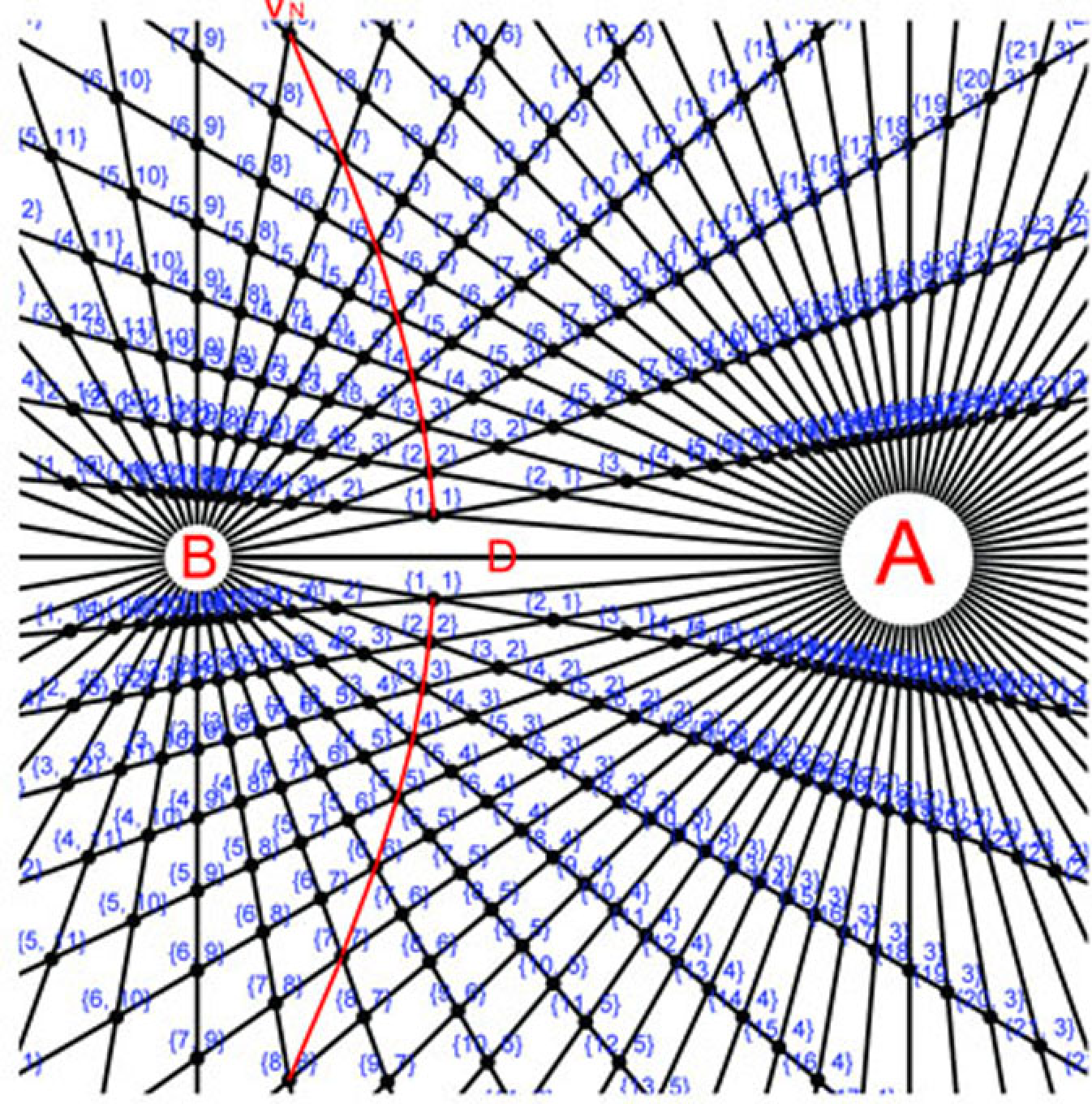
With respect to the bi-Radial coordinate system it is far more revealing to use a coordinate system who’s symmetry is similar to the phenomenon being analysed, in this case bi-polar force fields. As referenced above the bi-radial matrix is neither man made or arbitrary. The numbering of the rays is implied in the symmetry of the matrix. In diagram 3A as the poles A and B are opposite each other the rays are numbered in opposite directions. The D segment being the base line has the implied value of zero. Also there are two opposite hemispheres in the bi-radial matrix-the upper and lower hemisphere. Hence the rays in the lower hemisphere below the D segment are numbered in the opposite direction then the rays in the upper hemisphere. From this numbering of the rays in diagram 3A the resulting set of bi-radial coordinates are assigned to each node. In this case the number of rays from each pole is 24. Bear in mind when describing large scale masses the number of rays can be enormous-exceeding the screen resolution and our our optical resolution. The bi-radial equivalency principle allows smaller ray counts to be used and is covered elsewhere.
From diagram 3B we can see the quantized angles represent quantized units of time and the line segments along the rays represent discreet non-quantized spatial units. This clarifies the components of the space time network. Also we can examine a specific line segment such as {3,5},{4,5}. From the reference system of pole A this segment traverses a single quantized unit of time from ray 3 to ray 4 while moving slightly further from pole A. From the reference frame of pole B this same line segment traverse a unit of space along ray 5. Hence in the bi-radial matrix the very same phenomenon has different properties depending on the reference system. In any case we define the coordinates {X,Y} where X corresponds to the ray number from pole A and Y corresponds to the ray number from pole B. Each of the coordinates {X,Y} are thus time coordinates.
We can further analyze both attraction and repulsion lines using the bi-radial coordinate system.
We continue the analysis with the repulsion lines. Diagram 5 shows the repulsion lines with the bi-radial coordinates. We can observe that the difference of the coordinates on any repulsion line equals a constant. Take for example the first repulsion line in the upper right quadrant the coordinates are: {5,4}, {4,3}, {3,2},{2,1}. The formula for any given repulsion line is thus:
X-Y=K
Equation 4
Among other things we see that the phenomenon of attraction lines in the bi-radial matrix is associated with the operator of addition and the phenomenon of repulsion lines is associated with the operator
of subtraction. Also note that while the phenomenon of attraction is considered the “opposite” of repulsion the geometric orientation of the repulsion lines is not diametrically opposed but rather oriented at 90°
with respect to the D segment. It will be shown there are other hidden field structures within the bi-radial matrix associated with the operators of division and multiplication. In part one of this series previously
published regarding the initial connection algorithms the first one is to find the paths of “shortest distance” from pole A and B passing through the unoccupied nodes. Space is considered an electrical insulator.
Since the attraction lines are traversing the shortest possible distance from pole A to pole B through space they are thus traveling the path of least resistance. This corresponds to electricity. The aggregate of this attraction lines correspo0nds to magnetism.
The second connection algorithm relates to the paths starting from poles A and B passing within the closest proximity to the vertical axis “V”. Once we recognize time as angular displacement we can describe
the various field structures in terms of space and time. The bi-radial coordinate system applies to the gravitational equilibrium zone. We can further the analyses of the gravitational equilibrium zone using the bi-radial
coordinate system.
Diagram 6B
It is revealing to consider diagrams 6A and 6B in light of Lee Smolin’s description of Space”: “A useful metaphor arising in several approaches to quantum gravity is to imagine that space is not continuous but a lattice of discrete points...”. The bi-radial matrix lends itsewlf to a variety of physical interpretations. This includes electromagnetic and gravitational fields. Could then the nodes represent gravitons or “magnetons”, i.e. particles of magnetic force?
There are several other relationships within the bi-radial matrix to be covered in future articles.
Summary
A geometric definition of time based on established astronomical data and the relationship between space and time are further defined with respect to the fundamental equation of motion V=S/T. From here time and space were shown to have specific geometric components within the bi-radial matrix clarifying the resulting space time network therein. By introducing the bi-radial coordinate system the magnetic attraction and repulsion fields and gravitational fields were further analysed. Fundamental equations were derived to further the analysis. The concept of a quantum time potential was introduced as part of a quantum geometry applied to gravitation and electromagnetism. Further properties including the bi-radial equivalency principle and bi-radial scaling mechanism will be covered in future articles relating gravitation to the microscopic scale.
Remaining Sections of program Code
Remaining Sections of program Code
Biradial Plot Functions
Biradial Plot Functions
Begin Package
Begin Package
Usage Statements
Usage Statements
Begin Private
Begin Private
makeBRMPlot
makeBRMPlot
Inner Functions
Inner Functions
Package footer
Package footer
Vector Geometric Functions
Vector Geometric Functions
Begin Package
Begin Package
Usage Statements
Usage Statements
Begin Private
Begin Private
Vector Geometric Functions
Vector Geometric Functions
Package footer
Package footer