Before diving in, keep these key terms in mind: eigenvalue, eigenstate (or eigenmode), and wave equation. Now, let’s jump in.
Think about it: the theory is called “quantum”. So whatever “quantum” or “quantization” means, it must be the defining characteristic of this theory. In fact, the process of quantizing has been remarkably successful across various domains—except for gravity. That remains one of the most profound open questions in science: should we be “quantizing gravity” or “gravitizing quantum”?
Putting this open question aside for now, let’s focus on the core idea of “quantized quantities”. According to quantum theory, certain physical properties can only take on specific discrete values, usually determined by constraints on the system. While continuous values are possible in some cases, the defining feature of quantum mechanics is its “discrete nature”.
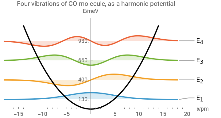
For instance, the energy of an electron confined within a region, say an atom, can only assume specific, quantized values—not just any arbitrary value. This was one of the great puzzles that quantum founders encountered. A key piece of evidence came from atomic spectra: atoms emit discrete spectral lines rather than a continuous spectrum (like a rainbow). These distinct lines correspond to quantized electron energies, revealing the fundamental departure of quantum theory from classical expectations.
Think about it: the theory is called “quantum”. So whatever “quantum” or “quantization” means, it must be the defining characteristic of this theory. In fact, the process of quantizing has been remarkably successful across various domains—except for gravity. That remains one of the most profound open questions in science: should we be “quantizing gravity” or “gravitizing quantum”?
Putting this open question aside for now, let’s focus on the core idea of “quantized quantities”. According to quantum theory, certain physical properties can only take on specific discrete values, usually determined by constraints on the system. While continuous values are possible in some cases, the defining feature of quantum mechanics is its “discrete nature”.
For instance, the energy of an electron confined within a region, say an atom, can only assume specific, quantized values—not just any arbitrary value. This was one of the great puzzles that quantum founders encountered. A key piece of evidence came from atomic spectra: atoms emit discrete spectral lines rather than a continuous spectrum (like a rainbow). These distinct lines correspond to quantized electron energies, revealing the fundamental departure of quantum theory from classical expectations.

Mathematically, these allowed values (such as the specific spectral lines in the example above) arise from a fundamental mathematical relationship known as the eigenvalue equation. The specific allowed values themselves are called eigenvalues, while the corresponding mathematical entities that describe the system’s state at those eigenvalues are known as eigenstates or eigenmodes.
Determining the eigenmodes and eigenvalues of various physical systems remains a crucial and ongoing computational challenge in science. Even today, researchers devote significant effort to solving these problems, as they play a key role in understanding everything from quantum mechanics to material properties and wave phenomena.
Determining the eigenmodes and eigenvalues of various physical systems remains a crucial and ongoing computational challenge in science. Even today, researchers devote significant effort to solving these problems, as they play a key role in understanding everything from quantum mechanics to material properties and wave phenomena.
But how do we find eigenmodes? Do they have classical counterparts? Interestingly, eigenmodes closely resemble the concept of standing waves in classical mechanics.
Consider the classical case of a drumhead, a two-dimensional membrane stretched over a circular frame. When you strike the drum, vibrations travel across the membrane, reflecting off the fixed circular edge and interfering with incoming waves from the center. When the interference is just right, a standing wave pattern emerges. These standing waves represent the natural modes of oscillation for the drum, which we call eigenmodes. During vibration, certain points remain stationary, known as nodes, while other points experience maximum vibration, called antinodes. The fixed edge of the drum, which does not move, serves as a boundary condition, meaning the displacement of the membrane is zero at that boundary.
The vibrations of the drumhead are described by a fundamental equation called the wave equation, which governs how the displacement of the drumhead evolves in space and time. A stationary wave, or standing wave, is a solution to this equation, appearing to stay in place rather than traveling freely. This type of wave exhibits both spatial and temporal variations. The spatial aspect determines the shape of the wave, including the locations of nodes and antinodes, while the temporal aspect describes how the wave oscillates over time. The peaks and troughs of the wave shift as time progresses, while the overall pattern remains stable, revealing the fundamental nature of eigenmodes in classical systems.
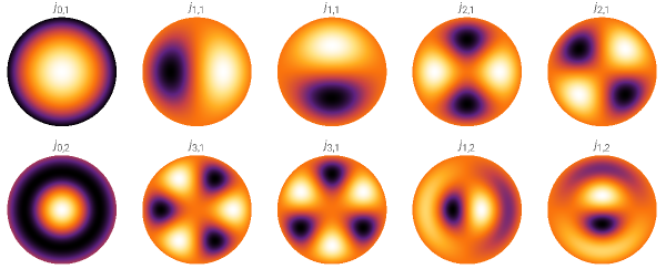
Let’s consider 10 eigenmodes of a circular drum with a radius of 1. For simplicity, we set the wave speed within the drum to 1. The labels for each mode correspond to the eigenvalues (the frequency of each wave). Mathematically, these are the zeros of the Bessel function, a fancy special function with many applications in both classical and quantum theories.
Out[]=
We can also freeze time (drop the time-dependent part) and focus only on the spatial aspect. The corresponding density plot would show the spatial patterns of eigenmodes.
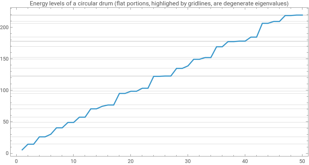
From this classical analysis, we learn that the frequencies of stationary waves are discrete. This means the frequencies cannot take just any value, but only specific ones. In some cases (e.g., look at the 2nd and 3rd waves, or the 4th and 5th), different waves correspond to the same frequency. This is called degeneracy, which has many interesting consequences in quantum theory (e.g., molecular resonance structures). The degenerate cases appear as flat portions on the graph (whenever there is a flat portion, two or more eigenmodes share the same eigenvalue).
From this classical analysis, we learn that the frequencies of stationary waves are discrete. This means the frequencies cannot take just any value, but only specific ones. In some cases (e.g., look at the 2nd and 3rd waves, or the 4th and 5th), different waves correspond to the same frequency. This is called degeneracy, which has many interesting consequences in quantum theory (e.g., molecular resonance structures). The degenerate cases appear as flat portions on the graph (whenever there is a flat portion, two or more eigenmodes share the same eigenvalue).
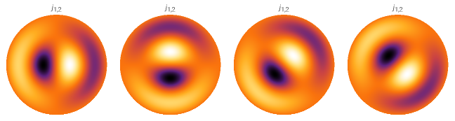
We will explore degenerate cases and their significance in a separate post. Briefly, if two eigenmodes share the same energy, any linear combination of them will also have the same energy, as seen in the examples below. While this may seem like a trivial property, it has profound fundamental implications, including the Schrödinger’s cat paradox. We will revisit this topic in another post.
For the drumhead example we discussed, the mathematical connection between classical and quantum theory is striking: eigenmodes and eigenvalues align with the classical case because the underlying eigenvalue relationship remains the same. So, what are the differences?
The physical correspondence for quantum waves is fundamentally different. A quantum wave is not directly observable; rather, it serves as a mathematical tool to describe observations, whereas classical waves can be directly seen. The interpretation of a quantum waves (i.e., quantum states) remains a subject of debate, though scientists widely agree on how to use it computationally.
Another key difference lies in time evolution. In quantum mechanics, if a system starts in a stationary state, its observable properties remain time-independent. In contrast, classical waves undergo time-dependent oscillations, forming nodes and antinodes, as we saw in the vibration of drumhead above.
Despite these differences, classical wave phenomena and quantum theory share striking similarities. When Schrödinger formulated his equation, he initially believed its solutions described real waves. Though this turned out to be incorrect, the mathematical resemblance persists. This is why Schrödinger’s equation is often called the quantum wave equation, and its solutions are referred to as wave functions.
This mathematical similarity suggests common features such as interference (due to wave superposition), evanescent waves (linked to quantum tunneling), and superoscillation, among other wave-like behaviors. However, one must always remember that the time-dependent behavior of quantum and classical waves differs significantly, though there are some similarities in limiting cases (such paraxial waves). More importantly, the fundamental distinction lies in their physical interpretation and implications—a difference that has fueled debates among scientists, even as they continue to apply quantum theory in practice.
In the next post, we’ll delve deeper into more quantum features and explore how they diverge from classical expectations. A longstanding debate is the wave-particle duality, which we will discuss next time. Here’s a sneak peek into the next post:
Out[]=
Appendix (codes)
Appendix (codes)
CITE THIS NOTEBOOK
CITE THIS NOTEBOOK
What is quantization? Eigenvalues, wave equations, and the physical interpretation of quantum states
by Mohammad Bahrami
Wolfram Community, STAFF PICKS, February 6, 2025
https://community.wolfram.com/groups/-/m/t/3383404
by Mohammad Bahrami
Wolfram Community, STAFF PICKS, February 6, 2025
https://community.wolfram.com/groups/-/m/t/3383404