Concentration profile for a tubular reactor with axial dispersion
Authors: Housam BINOUS and Ahmed Bellagi
Concentration profile for a tubular reactor with axial dispersion
Authors: Housam BINOUS and Ahmed Bellagi
Authors: Housam BINOUS and Ahmed Bellagi
A first order chemical reaction is taking place in a tubular chemical reactor : A → B
We assume that the flow is turbulent and that some axial dispersion is occurring .
The determination of the concentration profile in the reactor turns out to be a split boundary condition problem that is solved in the present notebook using four different approaches . The governing equations are given below (reproduced from textbook by Fred Ramirez (Computational Methods for Process Simulation, Second Edition, 1997, Butterworth-Heinemann, Oxford).
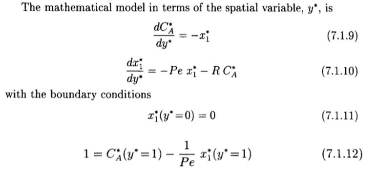
In what follows, we will assume that Pe=100 and R=200 where Pe is the Peclet and R a dimensionless reaction rate group.
1- The first approach is given by Professor Ramirez.
2- The second method is based on the shooting method developed by Professor Brian Higgins (Chemical Engineering Department, University of California, Davis).
3- The third method is a direct computation of the concentration profile using NDSolve.
4- The fourth method is based on shifted-Legendre orthogonal collocation.
We will see that all four methods give the same results .
Acknowledgement :
This problem was presented by W. F. Ramirez in Computational Methods for Process Simulation, 2ed Ed., 1997, Butterworth-Heinemann, Oxford.
This problem was presented by W. F. Ramirez in Computational Methods for Process Simulation, 2ed Ed., 1997, Butterworth-Heinemann, Oxford.
In[]:=
Off[General::"spell1"]
Guessing the value of CA[y=0] by two methods
First Method inspired by Professor Fred Ramirez
In[]:=
CA0=0.5;
In[]:=
delta=10;
In[]:=
i=1;
In[]:=
While[delta>0.0001,{sol=NDSolve[{D[CA[y],{y,1}]-x1[y],D[x1[y],{y,1}]-100x1[y]-200CA[y],x1[0]0,CA[0]CA0,D[f1[y],{y,1}]-f2[y],D[f2[y],{y,1}]-200f1[y]-100f2[y],f1[0]==1,f2[0]==0},{CA[y],x1[y],f1[y],f2[y]},{y,0,1}],delta=((1-CA[y]+0.01x1[y])/(-f1[y]+0.01f2[y])/.sol/.y1)[[1]],CA0+=-delta,i=i+1,Print[i," ",delta]}]
2 0.359408
3 -1.72529×
-9
10
In[]:=
CA0
Out[]=
0.140592
Second Method inspired by Professor Brian Higgins (U C Davis)
In[]:=
CA0=.
In[]:=
SOLD[CA0_]:=NDSolve[{D[CA[y],{y,1}]-x1[y],D[x1[y],{y,1}]-100x1[y]-200CA[y],x1[0]0,CA[0]CA0},{CA[y],x1[y]},{y,0,1}]
In[]:=
yend[CA0_?NumericQ]:=1-(CA[y]/.SOLD[CA0]/.y1)+(0.01x1[y]/.SOLD[CA0]/.y1)
In[]:=
FindRoot[yend[CA0]0,{CA0,0.5},MaxIterations1000]
Out[]=
{CA00.140592}
Plotting the concentration profile
In[]:=
First[CA[y]/.SOLD[0.140592]/.y0]
Out[]=
0.140592
In[]:=
f=CA[y]/.SOLD[0.140592]
Out[]=
InterpolatingFunction[y]


In[]:=
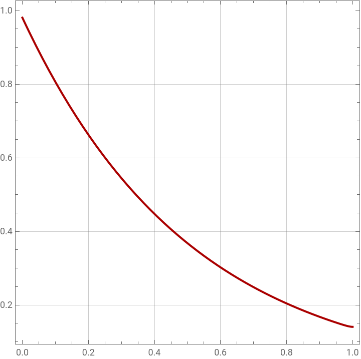
plt1=Plot[(f/.y1-x),{x,0,1},PlotStyle{Thick,Darker@Red},AspectRatio->1,GridLines->Automatic,Frame->True]
Out[]=
Third Method using NDSolve
Indeed, NDSolve can often solve boundary value problems
Indeed, NDSolve can often solve boundary value problems
In[]:=
solbvp=NDSolve[{D[CA[x],{x,2}]-100D[CA[x],{x,1}]-200CA[x]0,CA'[1]0,1CA[0]-0.01CA'[0]},{CA[x]},{x,0,1}]
Out[]=
CA[x]InterpolatingFunction[x]

Plotting the concentration profile
In[]:=
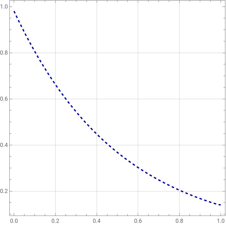
plt2=Plot[Evaluate[CA[x]/.solbvp],{x,0,1},PlotStyle{Thick,Dashed,Darker@Blue},AspectRatio->1,GridLines->Automatic,Frame->True]
Out[]=
In[]:=
CA[x]/.solbvp/.x1
Out[]=
{0.140592}
Fourth Method using orthogonal collocation using shifted-Legendre polynomials
In[]:=
Np=15;
In[]:=
sol=Solve[JacobiP[Np-2,0,0,2x-1.]0,x]
Out[]=
{{x0.00790847},{x0.0412008},{x0.099211},{x0.178825},{x0.275754},{x0.384771},{x0.5},{x0.615229},{x0.724247},{x0.821174},{x0.90079},{x0.958799},{x0.992092}}
In[]:=
tbl=Select[Table[x/.sol[[i]],{i,1,Length[sol]}],#>0&];x[Np]=1.0;x[1]=10^-20;For[i=2,i<Np,{x[i]=tbl[[i-1]],i++}];
In[]:=
Q=Chop[Table[Table[x[j]^(i-1),{i,1,Np}],{j,1,Np}]];IQ=Inverse[Q]//Quiet;Ci=Chop[Table[Table[(i-1)x[j]^(i-2),{i,1,Np}],{j,1,Np}]];A=Ci.IQ;
In[]:=
A//MatrixForm
Out[]//MatrixForm=
-182.656 | 202.547 | -25.8347 | 8.58099 | -4.09272 | 2.38234 | -1.58497 | 1.16771 | -0.937069 | 0.812568 | -0.760547 | 0.774683 | -0.883883 | 1.26465 | -0.780268 |
-79.0225 | 63.1965 | 19.8815 | -5.7683 | 2.6356 | -1.50268 | 0.98733 | -0.721199 | 0.575127 | -0.496372 | 0.462967 | -0.470385 | 0.535796 | -0.765918 | 0.472461 |
23.3577 | -46.0837 | 12.5302 | 13.3608 | -4.65294 | 2.34394 | -1.41871 | 0.972717 | -0.736895 | 0.610049 | -0.550575 | 0.545744 | -0.611237 | 0.865682 | -0.532845 |
-11.2487 | 19.6596 | -20.9192 | 4.32671 | 11.2326 | -4.7538 | 2.85383 | -2.02983 | 1.61458 | -1.40241 | 1.31951 | -1.35156 | 1.54895 | -2.22205 | 1.37184 |
6.41783 | -10.8492 | 9.27563 | -13.5909 | 1.66595 | 10.0055 | -4.7106 | 3.09204 | -2.37818 | 2.03372 | -1.89899 | 1.93773 | -2.21656 | 3.17714 | -1.96115 |
-4.6651 | 7.7349 | -6.00251 | 6.6246 | -10.8914 | 0.908285 | 8.9824 | -4.39029 | 2.98702 | -2.38925 | 2.14219 | -2.13082 | 2.39996 | -3.41277 | 2.1028 |
3.52647 | -5.79308 | 4.30197 | -4.27369 | 5.31045 | -9.43236 | 0.363971 | 8.67309 | -4.44474 | 3.17636 | -2.68634 | 2.58427 | -2.85546 | 4.022 | -2.47291 |
-2.76494 | 4.51829 | -3.27517 | 3.08708 | -3.44061 | 4.61691 | -8.70882 | -0.0809496 | 8.87357 | -4.7908 | 3.63141 | -3.30675 | 3.54814 | -4.92793 | 3.02056 |
2.22287 | -3.62072 | 2.58644 | -2.36544 | 2.49337 | -2.9972 | 4.27139 | -8.49902 | -0.544995 | 9.62736 | -5.5281 | 4.52764 | -4.62049 | 6.27358 | -3.82668 |
-1.81288 | 2.94672 | -2.08536 | 1.87181 | -1.91003 | 2.16943 | -2.76972 | 4.16728 | -8.74556 | -1.16802 | 11.1855 | -6.9716 | 6.44125 | -8.3997 | 5.08088 |
1.48239 | -2.40618 | 1.69238 | -1.50087 | 1.501 | -1.64975 | 1.99109 | -2.68717 | 4.27325 | -9.51906 | -2.22354 | 14.2554 | -10.1214 | 12.1353 | -7.22289 |
-1.19486 | 1.93769 | -1.35738 | 1.19444 | -1.17946 | 1.27081 | -1.48575 | 1.89921 | -2.71715 | 4.6065 | -11.0686 | -4.51696 | 21.1552 | -20.0129 | 11.4692 |
0.916712 | -1.48578 | 1.03821 | -0.909214 | 0.890935 | -0.948709 | 1.08932 | -1.3528 | 1.8411 | -2.82611 | 5.21849 | -14.0481 | -11.6416 | 44.7209 | -22.5033 |
-0.595773 | 0.965317 | -0.673652 | 0.588487 | -0.574381 | 0.607998 | -0.691895 | 0.847461 | -1.12763 | 1.6625 | -2.82254 | 5.99507 | -20.1741 | -62.7494 | 78.7425 |
0.949326 | -1.53808 | 1.07304 | -0.936864 | 0.913601 | -0.965784 | 1.09687 | -1.33944 | 1.77365 | -2.59323 | 4.33219 | -8.85986 | 26.1784 | -203.06 | 182.976 |
Hence, we get a value in close agreement with the results found above (i.e., CA(@ y=0) = 0.140611)
Hence, we get a value in close agreement with the results found above (i.e., CA(@ y=0) = 0.140611)
Comparing concentration profiles obtained using the various methods presented above.
A visual check confirms that all methods agree closely.
A visual check confirms that all methods agree closely.