The study of the dynamics of the discrete Klein - Gordon equation (DKG) with friction is given by the equation:
̈
U
n
U
n+1
U
n
U
n-1
U
n
′
W
U
n
In the above equation, describes the potential function:
W
W()-+
U
n
2
w
d
2
2
U
n
β
2
w
d
4
4
U
n
to which every coupled unit adheres. In Eq. (1), the variable (t) is the unknown displacement of the oscillator occupying the -th position of the lattice, and is the discretization parameter. We denote by the distance between the oscillators of the lattice. The chain (DKG) contains linear damping with a damping coefficient , while is the coefficient of the nonlinear cubic term.
U
n
U
n
n
k
-2
h
h
δ>0
β
For the DKG chain (1), we will consider the problem of initial-boundary values, with initial conditions
U
n
U
n,0
U
n
U
n,1
K+2
R
and Dirichlet boundary conditions at the boundary points -L/2 and L/2, that is,
x
0
x
K+1
U
0
U
K+1
Therefore, when necessary, we will use the short notation for the one-dimensional discrete Laplacian
Δ
d
{U}
Δ
d
n∈Z
U
n+1
U
n
U
n-1
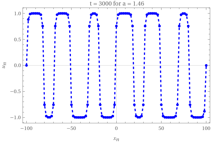
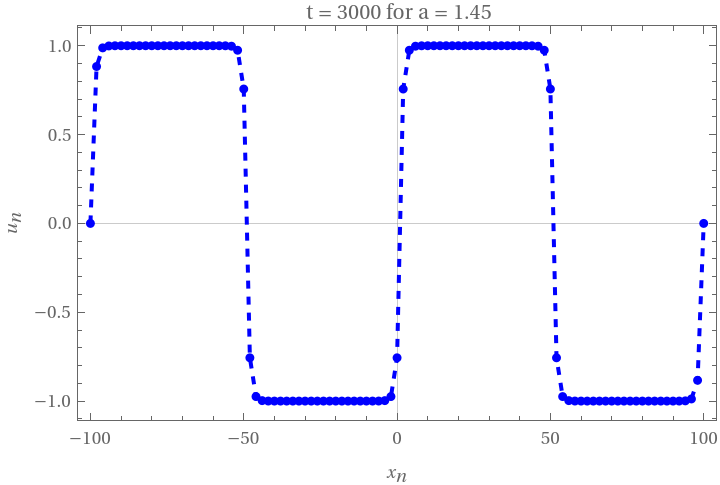
In this note book, we investigate numerically the dynamics of the system (1)-(2)-(3). Our first aim is to conduct a numerical study of the property of Dynamic Stability of the system, which directly depends on the existence and linear stability of the branches of equilibrium points.For the discussion of numerical results, it is also important to emphasize the role of the parameter . By changing the time variable , we rewrite Eq. (1) in the form-U+-β, t>0, , hδThe change in the scaling of the lattice parameter of the problem makes it important to comment here on the nature of the continuous and anti-continuous limit. For the anti-continuous limit, we need to consider the case in Eq. (1) where ∞. In the case of nonlinearity present in the governing equations, the continuous limit needs to be taken as well. On the other hand, for small values of the parameter, the system becomes significant. However, because of the model we consider, we take the asymptotic linear limit as 0.
2
ω
d
t
t
h
̈
U
n
Δ
d
δ
U
n
2
Ω
d
U
n
3
U
n
2
Ω
d
2
h
2
ω
d
δ
2
ω
d
2
ω
d
We consider spatially extended initial conditions of the form :
U
n
U
n,0
jπhn
L
where is the distance of the grid and is the amplitude of the initial condition .We also assume zero initial velocity:
h
L
K+1
a>0
U
n
U
n,1
In[]:=
ClearAll["Global`*"]
List of different values for a:
aList={2,1.95,1.9,1.85,1.82,1.81,1.55,1.46,1.45};
Mode number:
j=4;
Length of the system:
L=200;
Characteristic frequency:
omegad=1;
Nonlinearity parameter:
beta=1;
Damping coefficient:
delta=0.05;
Spatial grid spacing:
h=2;
Spatial points:
grid=Range[-L/2,L/2,h];
Number of spatial points:
k=Length[grid];
omegad2=(h^2)*omegad^2;
deltaHat=h*delta;
Maximum time:
tmax=3000;
Generate initial plot for a=2 :
var=Table[u[i][t],{i,k}];
eqs=Table[u[i]''[t]-(u[i+1][t]+u[i-1][t]-2u[i][t])+deltaHatu[i]'[t]-omegad2(u[i][t]-betau[i][t]^3)==0,{i,2,k-1}];
bc={u[1][t]==0,u[1][k]==0};
ic=Join[Thread[var==2Sin[4Pigrid/L]]/.t->0,Table[u[i]'[0]==0,{i,2,k-1}]];
sol=NDSolve[Join[eqs,{u[1]'[t]==0,u[k]'[t]==0},ic],var,{t,0,tmax}];
initialPlot=ListPlot[Transpose[{grid,var/.sol[[1]]/.t->0}],FrameLabel->{"",""},PlotLabel->" a t = 0 for a = 2",PlotTheme->"Scientific",PlotStyle->{Red,PointSize[Medium]}];
x
n
u
n
Solve the equations and generate plots for each value of a :
plots=Table[Module[{var,eqs,bc,ic,sol,finalPlot},var=Table[u[i][t],{i,k}];eqs=Table[u[i]''[t]-(u[i+1][t]+u[i-1][t]-2u[i][t])+deltaHatu[i]'[t]-omegad2(u[i][t]-betau[i][t]^3)==0,{i,2,k-1}];bc={u[1][t]==0,u[1][k]==0};ic=Join[Thread[var==aSin[4Pigrid/L]]/.t->0,Table[u[i]'[0]==0,{i,2,k-1}]];sol=NDSolve[Join[eqs,{u[1]'[t]==0,u[k]'[t]==0},ic],var,{t,0,tmax}];finalPlot=Show[ListPlot[Transpose[{grid,var/.sol[[1]]/.t->tmax}],FrameLabel->{"",""},PlotLabel->" t = 3000 for a = "<>ToString[a],PlotTheme->"Scientific",PlotStyle->{Blue,PointSize[Medium]}],ListLinePlot[Transpose[{grid,var/.sol[[1]]/.t->tmax}],{PlotStyle->{Blue,Dashed}}]];finalPlot],{a,aList}];
x
n
u
n
Display the initial plot and the final plots in a grid with 2 plots per row:
Grid[Partition[Prepend[plots,initialPlot],2]]
Out[]=
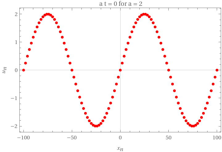
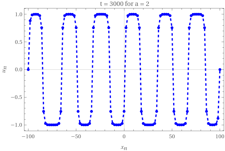
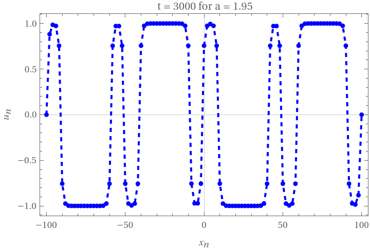
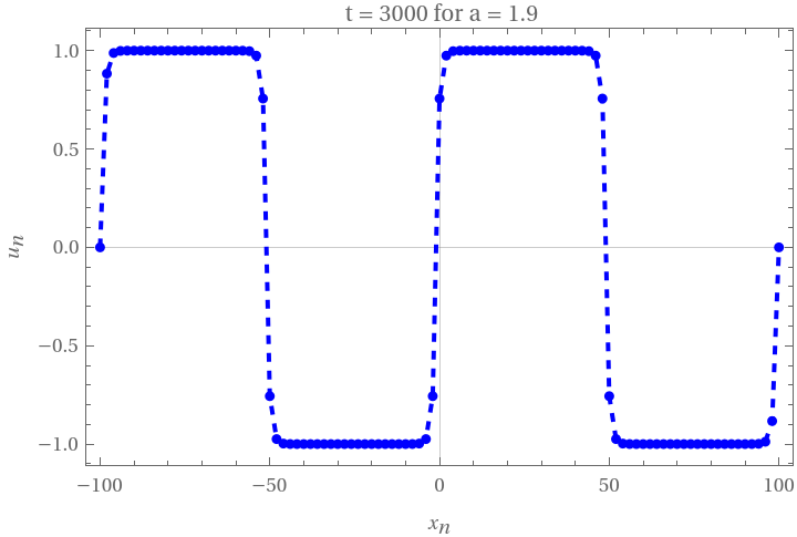
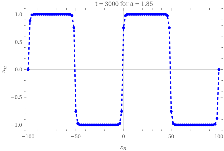
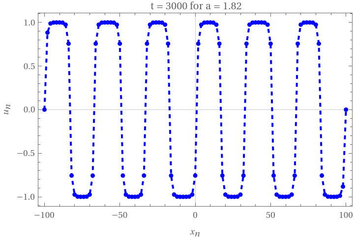
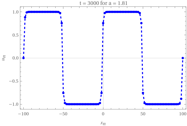
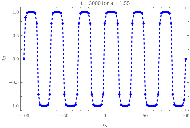
Evolution of Spatially Localized Initial Conditions
Evolution of Spatially Localized Initial Conditions
Now we examine the role of damping in the structure of the branches of equilibrium points . In this study, we consider localized initial conditions of the form :
U
n
U
n,0
L
2
where is the distance between the nodes, and is the amplitude . We assume zero initial velocity
h
L
K+1
a>0
(0)0.
U
n
U
n,1
We also note that if we consider an infinite chain, the initial conditions satisfy the Dirichlet boundary conditions only asymptotically . However, since the smallest half - length of the chain has been set to $ $, the error is of the order of , which does not affect numerical computations . Figure 2.13 shows the dynamics of the initial condition (2.143) for parameters : 1,K99,L200, and . In the first image , we observe the profile of the initial condition . The subsequent images show the dynamics of the system for different values of the damping force . For , the convergence takes place at the equilibrium point ∈ which is the basic state .
(1)
L/2100
-44
10
2
ω
0
β1
δ0.1,0.05,0.01
δ0.1
Φ
1
C
1
Amplitude of the initial condition:
Mode number:
Length of the system:
Characteristic frequency:
Nonlinearity parameter:
List of damping coefficients:
Spatial grid step size:
Spatial points:
Number of spatial points:
Scaled frequency:
Maximum time for simulation:
Variables for each grid point:
Initial conditions:
Function to solve the system for a given delta:
Solve the system for each value of delta in deltaList:
Visualization:
Display all plots:
Amplitude of the initial condition:
Length of the system:
Characteristic frequency:
Nonlinearity parameter:
Damping coefficient:
Spatial grid:
Spatial points:
Number of spatial points:
Discretization parameter:
Scaled parameters:
Maximum time:
Initial positions:
Parameters:
Amplitude of the initial condition:
Length of the system:
Characteristic frequency:
Nonlinearity parameter:
Damping coefficient:
Spatial grid:
Spatial points:
Number of spatial points:
Discretization parameter:
Scaled parameters:
Maximum time:
Initial positions:
Acknowledgements
Acknowledgements
I would like to express my deepest gratitude to my advisor, Prof . Nikolaos Karachalios from the Department of Mathematics, University of Thessaly . Prof . Karachalios and I chose this project together, and his unwavering support, guidance, and valuable feedback have been instrumental in helping me evaluate my knowledge of ODEs and dynamical systems .
I am also immensely thankful to Dr . Alexander Trounev from the Department of Computer Technology and Systems, Kuban State Agrarian University, Russia . Dr . Trounev provided crucial assistance when I faced difficulties with my code and took the time to explain what steps to take, greatly enhancing my understanding and progress .
I am also immensely thankful to Dr . Alexander Trounev from the Department of Computer Technology and Systems, Kuban State Agrarian University, Russia . Dr . Trounev provided crucial assistance when I faced difficulties with my code and took the time to explain what steps to take, greatly enhancing my understanding and progress .
Refferences
Refferences
1
.2
.S. W. Englander, N. R. Kallenbach, A. J. Heeger, J. A. Krumhansl, and S. Litwin, Nature of the open state in long polynucleotide double helices: possibility of soliton excitations, Proceedings of the National Academy of Science USA, 77 (12) (1980) 7222-7226.
CITE THIS NOTEBOOK
CITE THIS NOTEBOOK
Numerical Simulation of the Discrete Klein-Gordon Equation: A Study on Damped,Driven Nonlinear Waves
by Athanasios Paraskevopoulos
Wolfram Community, STAFF PICKS, June 11, 2024
https://community.wolfram.com/groups/-/m/t/3190706
by Athanasios Paraskevopoulos
Wolfram Community, STAFF PICKS, June 11, 2024
https://community.wolfram.com/groups/-/m/t/3190706