We consider a composite domain made up of a large rectangle with a small rectangular branch attached to it. The focus is on the eigensystem problem for the Laplacian with Dirichlet boundary conditions, where the goal is to understand why and when an eigenfunction shows a high probability density in the small branch. If the branch were considered on its own, it would have its own set of eigenvalues. When an eigenvalue of the full composite domain is very close to one of the branch’s eigenvalues, the branch “resonates” with that mode. Due to the weak connection between the main rectangle and the branch, this near-resonance causes the eigenfunction to localize in the branch, resulting in a concentration of the probability density there. This phenomenon is typically analyzed using perturbation methods and asymptotic matching techniques, but here we explored it numerically. Another interesting feature that we explored in the exponential decay of spatial density function within small rectangle, which is observed for eigensystems that the branch do NOT resonates with that mode. Of course, this analysis can be generated to arbitrary shapes, and 3D, but here we kept it simple to 2D and rectangle shapes.
Relevant literature: Delitsyn, A., Nguyen, B. & Grebenkov, D. Exponential decay of Laplacian eigenfunctions in domains with branches of variable cross-sectional profiles. Eur. Phys. J. B 85, 371 (2012). https://doi.org/10.1140/epjb/e2012-30286-8
https://arxiv.org/pdf/1109.3408
https://arxiv.org/pdf/1109.3408
Find eigenstates and eigenvalues
Find eigenstates and eigenvalues
Create a region with a branch:
In[]:=
Δ=1;δ=.25;Graphics[{FaceForm[],EdgeForm[Black],r1=Rectangle[{0,0},{π,π}],r2=Rectangle[{π,π/2-δ/2},{π+Δ,π/2+δ/2}]},AspectRatio->Automatic,Axes->True]
Out[]=
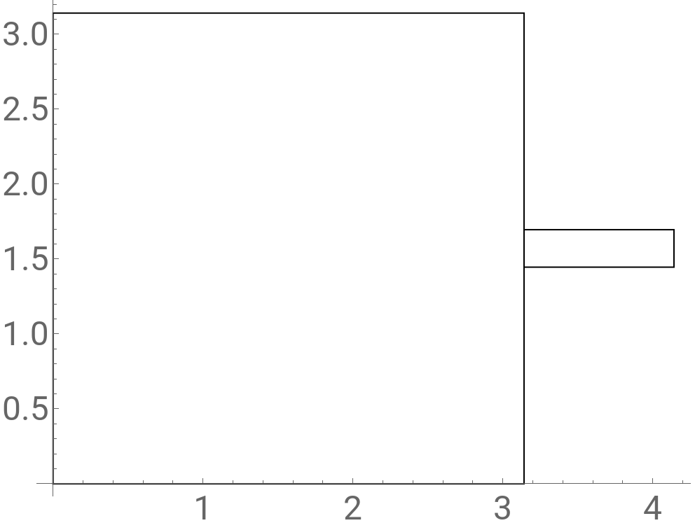
Merge them:
In[]:=
ℛ=RegionUnion[r1,r2]
Out[]=
Polygon


Find first 200 eigenvalues and eigenstates:
In[]:=
{vals,funs}=NDEigensystem[{-Laplacian[u[x,y],{x,y}],DirichletCondition[u[x,y]0,True]},u[x,y],{x,y}∈ℛ,200,Method{"VectorNormalization"->True,"Eigensystem"{"Arnoldi","MaxIterations"10^6},"PDEDiscretization"{"FiniteElement",{"MeshOptions"{"MaxCellMeasure"0.001}}}}];
Visualization
Visualization
Visualize the corresponding spatial density:
In[]:=
imgs=Table[Show[ContourPlot[Abs[Evaluate[dt[[-1]]]]^2,{x,y}∈ℛ,PlotLabelToString[dt[[1]]]<>"-th level, with energy "<>ToString[dt[[2]]],Frame->False,Axes->False,PlotPoints100,ColorFunction"SunsetColors",AspectRatioAutomatic,PlotRange->All,ContourStyleNone,MaxRecursion0],Graphics[{FaceForm[],EdgeForm[Black],ℛ}]],{dt,Transpose[{Range[Length@vals],vals,funs}]}];
Numerical integration for probability of particle being on the small branch:
In[]:=
probR2=Quiet[NIntegrate[Abs[Evaluate@#]^2,{x,y}∈r2]]&/@funs;
Create a GIF:
In[]:=
Export[NotebookDirectory[]<>"Denisty.GIF",maxProb[[All,-1]]]
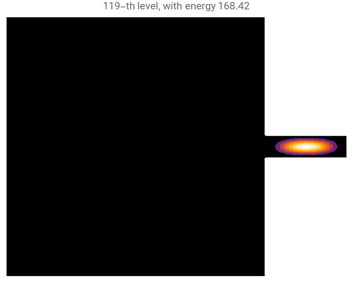
For cases with the exponential decay in the small branch, the density in the small branch cannot have any wavy feature which happens usually when the eigenmode is localized in the small branch (as some examples, look at the following density plots). Therefore, one can argue none of them fulfil the conditions needed for the exponential decay inside small rectangle.
A naive explanation for the localization could be this: it happens if the eigenvalue in the small branch is close to an eigenvalue of overall domain (both rectangles).
Find 20 eigenvalues in the small branch:
In[]:=
valsR2=NDEigenvalues[{-Laplacian[u[x,y],{x,y}],DirichletCondition[u[x,y]0,True]},u[x,y],{x,y}∈r2,200,Method{"VectorNormalization"->True,"Eigensystem"{"Arnoldi","MaxIterations"10^6},"PDEDiscretization"{"FiniteElement",{"MeshOptions"{"MaxCellMeasure"0.001}}}}];
Find closest overall eigenvalue to them ({prob in the small branch, eigenvalue in the small branch}->closest eigenvalue of overall domain):
In[]:=
AssociationMap[Nearest[valsR2,#[[-1]]]&,ReverseSortBy[Transpose[{probR2,vals}],First]][[;;30]]
Out[]=
{0.516122,168.42}{167.788},{0.280819,163.725}{167.788},{0.233519,186.842}{197.397},{0.197483,235.904}{246.746},{0.181551,197.062}{197.397},{0.175269,214.409}{197.397},{0.174099,194.599}{197.397},{0.162015,229.848}{246.746},{0.138317,249.535}{246.746},{0.117686,160.592}{167.788},{0.0921495,183.985}{197.397},{0.0884918,201.503}{197.397},{0.0810241,263.112}{246.746},{0.0752567,245.155}{246.746},{0.0729255,176.359}{167.788},{0.0687591,256.129}{246.746},{0.051731,204.244}{197.397},{0.0491672,169.422}{167.788},{0.0473237,223.256}{246.746},{0.036823,242.212}{246.746},{0.0351409,142.109}{167.788},{0.028228,193.291}{197.397},{0.0272273,219.25}{197.397},{0.0266065,180.352}{167.788},{0.0174666,268.649}{246.746},{0.0141096,151.982}{167.788},{0.00850473,128.554}{167.788},{0.00828719,260.937}{246.746},{0.00820156,120.893}{167.788},{0.00809227,156.762}{167.788}
Density plots for eigenmodes with max prob in the small branch:
In[]:=
ListAnimate[Column[{"Prob. in the small branch = "<>ToString[#1],#2}]&@@@ReverseSortBy[Transpose[{probR2,imgs}],First][[;;20]],AnimationRunning->False,SaveDefinitions->True]
Out[]=
Explore the potential decay in the small branch
Explore the potential decay in the small branch
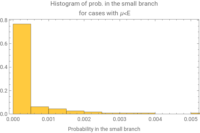
μ<En cases
μ<
E
n
μ is the min eigenvalue for cross sections in the branch (smaller rectangle here)
Eq 13 in https://arxiv.org/pdf/1109.3408
This is similar an example of wave cutoff and evanescent decay, as discussed in Jackson’s “Classical Electrodynamics”, Section 8.3.
ChatGPT explanation on this (classical case): https://chatgpt.com/share/679bd617-79d0-8006-b728-dc7a98f7a8a9
Eq 13 in https://arxiv.org/pdf/1109.3408
This is similar an example of wave cutoff and evanescent decay, as discussed in Jackson’s “Classical Electrodynamics”, Section 8.3.
ChatGPT explanation on this (classical case): https://chatgpt.com/share/679bd617-79d0-8006-b728-dc7a98f7a8a9
Min eigenvalue of 1D particle in a box (cross section
In[]:=
μmin=π^2/δ^2
Out[]=
157.914
Again, as I mentioned before, the reader should pay attention that cases with are cases for which the probability in the branch is really small (eg the max probability value is less than 4%)
μ<
E
n
Out[]=
Create a new dataset with eigenstate number, its value, the corresponding eigenstate, probability of being in the small branch, and corresponding plot, and sort them in terms of probability in the small branch:
In[]:=
dampedEigen=ReverseSortBy[Select[Transpose[{Range[Length@vals],vals,funs,probR2,imgs}],#[[2]]<μmin&],#[[-2]]&];
Add density plot within the small branch into the dataset:
In[]:=
dampedEigen=With[{branchCP=ContourPlot[Abs[Evaluate[#[[3]]]]^2,{x,y}∈r2,Frame->False,Axes->False,PlotPoints100,ColorFunction"SunsetColors",AspectRatioAutomatic,PlotRange->All,ContourStyleNone,MaxRecursion0]&/@dampedEigen},Flatten/@Transpose[{dampedEigen,branchCP}]];
Visualize corresponding densities:
In[]:=
Manipulate[GraphicsColumn[MapAt[Row[{"Prob. in the small branch = ",#}]&,dampedEigen[[n,{-3,-1,-2}]],{1}],ImageSize->Medium],Style["Eigenmodes with energy less than min energy of cross-sections in the small branch.\n The density plot at the top contains only small branch, and values are rescaled for that region only.",Bold,Medium],{{n,1,""},1,Length[dampedEigen],1},SaveDefinitions->True]
Out[]=
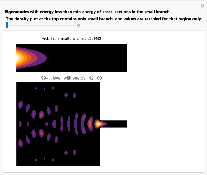
Take the first element (the one with the largest probability)
Calculate the density inside the small branch, across different cross sections (ie the red line in below graphics)
Densities along different cross-sections in the small branch (red lines in above visualization):
Normalize the result wrt the first value:
Another bound can be obtained for probability (the probability within the red region below):
Find the probabilities:
Normalize the result wrt the first one:
Compare numerical resuls with the bound:
Note that the formula is only a bound and it does not mean it fits the numerical result. Look at below example:
only a bound!
only a bound!
Note the cases above that bounds may look fitting the numerical data are only a special case. As said, those formulas are only provide an upper bound for the exponential damping. consider the following example.
Densities along cross sections of the small branch:
Normalize the result wrt the first value:
Another bound can be obtained for probability:
Probabilities along different regions within the small branch:
Normalize the result wrt the first one:
Compare numerical results with the bound:
CITE THIS NOTEBOOK
CITE THIS NOTEBOOK
Exponential decay of eigenstates in a branch
by Mohammad Bahrami
Wolfram Community, STAFF PICKS, February 7, 2025
https://community.wolfram.com/groups/-/m/t/3387401
by Mohammad Bahrami
Wolfram Community, STAFF PICKS, February 7, 2025
https://community.wolfram.com/groups/-/m/t/3387401