In this post I explain the difference between the why and the how of this theorem. The why is the theoretical proof using advanced algebraic techniques. Often this theorem is given as an easy corollary of Clebsch’s genus formula, a rather deep result. A somewhat easier proof is in Gerd Fischer’s Plane Algebraic Curves book (AMS, 2001). It uses the idea of effective divsors and is given by an indirect proof from Bézout’s theorem. In my book A numerical approach to Real Algebraic Curves with the Wolfram Language (Wolfram Media, 2018) I show that this can be made into a direct algorithmic proof, in the simple case, using only basic ideas. In other words, I explain the how. In this post I give an updated version of my algorithm as a Mathematica procedure. A nice feature of this approach is that this post should be readable even by those with no background at all in algebraic geometry. CITATION (original book): Barry H. Dayton (2018), A Numerical Approach to Real Algebraic Curves with the Wolfram Language. Wolfram Media, Inc. ISBN: 9781579550240. https://www.wolfram-media.com/products/dayton-algebraic-curves/
Amazon: https://a.co/d/eOn3RTP
Amazon: https://a.co/d/eOn3RTP
The Number of Singular points on a plane algebraic curve
The Number of Singular points on a plane algebraic curve
A theorem in plane algebraic curve theory says, loosely:
An irreducible algebraic plane curve of degree d has at most singularities.
(d-1)(d-2)
2
In this post I explain the difference between the why and the how of this theorem. The why is the theoretical proof using advanced algebraic techniques. Often this theorem is given as an easy corollary of Clebsch’s genus formula, a rather deep result. A somewhat easier proof is in Gerd Fischer’s
Plane Algebraic Curves book (AMS, 2001). It uses the idea of effective divsors and is given by an indirect proof from Bézout’s theorem. In my book A numerical approach to Real Algebraic Curves with the Wolfram Language (Wolfram Media, 2018) I show that this can be made into a direct algorithmic proof, in the simple case, using only basic ideas. In other words, I explain the how. In this post I give an updated version of my algorithm as a Mathematica procedure. A nice feature of this approach is that this post should be readable even by those with no background at all in algebraic geometry.
Plane Algebraic Curves book (AMS, 2001). It uses the idea of effective divsors and is given by an indirect proof from Bézout’s theorem. In my book A numerical approach to Real Algebraic Curves with the Wolfram Language (Wolfram Media, 2018) I show that this can be made into a direct algorithmic proof, in the simple case, using only basic ideas. In other words, I explain the how. In this post I give an updated version of my algorithm as a Mathematica procedure. A nice feature of this approach is that this post should be readable even by those with no background at all in algebraic geometry.
1. Definitions and basic facts on plane curves.
1. Definitions and basic facts on plane curves.
A bivariate polynomial in this post is a finite sum of monomials where are non-negative integers and, in this post could be a complex machine number although for most examples here they will be integers or rational fractions for readability and reuse. The total degree, often just called the degree, is the largest sum of for a monomial with non-zero coefficient. In case of machine number coefficients, a very small coefficient, say , would be considered zero.
a
i,j
i
x
j
y
i,j
thecoeffcient
a
i,j
i+j
Abs[]<
a
i,j
-12
10
For example, here is a polynomial drawn in blue above. In this case the degree is 5.
In[]:=
f=5.-2.5`x+0.5`+11.`--4-5.`y+7.5`xy-8.`y-3y+4y-4.5`-1.5`x-3+4.5`-3x+3++x-;
2
x
3
x
4
x
5
x
2
x
3
x
4
x
2
y
2
y
3
x
2
y
3
y
3
y
2
x
3
y
4
y
4
y
5
y
An algebraic plane curve is the solution set of the equation where is a bivariate polynomial. For display we might be thinking of solution in however for our main result we need the solution in . Algebraic geometers would want the solution in thecomplexprojectiveplane. I will discuss this case later in the post.
f=0
f
2
2
2
A bivariate polynomial or its curve is irreducible if it cannot be factored with coefficients in . The fundamental theorem of algebra says every one variable polynomial can be factored over but this is far from true for bivariate polynomials. In particular all reducible contain a singular point, usually many. Geometrically we see the blue curve above will be reducible because it contains a circle, a hyperbola and a line. An irreducible curve is expected to contain only one geometric figure but our picture is not showing a possible complex part.
A singular point of a curve is a point where there is no single tangent vector. In particular to be singular both the partial derivatives D[f,x], D[f,y] evaluated at the point should be zero. In our example above the point p below is singular because
A singular point of a curve is a point where there is no single tangent vector. In particular to be singular both the partial derivatives D[f,x], D[f,y] evaluated at the point should be zero. In our example above the point p below is singular because
In[]:=
p={0.7358898943575471`,1.399452058262947`}D[f,{x}]/.Thread[{x,y}->p]D[f,y]/.Thread[{x,y}->p]
Out[]=
{0.73589,1.39945}
Out[]=
-4.63984×
-12
10
Out[]=
-2.56577×
-11
10
the partial derivatives are effectively zero.
Here is some code to calculate the complex affine singular points. It is described in Chapter 5.3 of my Plane Curve Book. That lines 2,3 and 5,6 are the same is not a misprint.
In[]:=
complexSingularPoints2D[f_,u_,v_]:=Module[{a,b,sol1,sol2,solz},{a,b}=RandomComplex[{-1-I,1+I},2];sol1={u,v}/.NSolve[{f,aD[f,u]+bD[f,v]}];{a,b}=RandomComplex[{-1-I,1+I},2];sol2={u,v}/.NSolve[{f,aD[f,u]+bD[f,v]}];solz=Join[sol1,sol2];Flatten[Take[Select[Tally[solz,Norm[#1-#2]<.001&],#[[2]]>1&],All,1],1]]
2. Our theorem and method of attack.
2. Our theorem and method of attack.
We will prove a slightly easier version of the standard theorem by assuming all singular points are affine, not infinite and ignoring the multiplicity of the singular points.
Original Theorem : Suppose the plane curve f = 0 is irreducible of degree d, then f has no more than distinct affine singular points.
(d-1)(d-2)
2
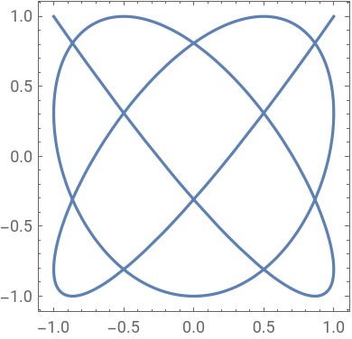
It should be mentioned that this bound is tight, Fischer shows that the Chebyshev curve of degree d is algebraic and actually has this number of singularities. This curve is built into Mathematica, for example for d =6 the curve has 10 singularities.
In[]:=
ParametricPlot[{ChebyshevT[5,t],ChebyshevT[6,t]},{t,-1,1},Axes->False,Axes->False,Frame->True,ImageSize->Small]
Out[]=
Typically books on algebraic geometry will give an indirect proof with the assumption that an irreducible curve has more thansingular points and deriving a contradiction. We can do a better job, we don’t assume it is irreducible we show how to factor a curve of degree d with more than this many singularities. That is we prove the contrapositive of the original theorem.
(d-1)(d-2)
2
Our Theorem: Suppose the plane curve f = 0 of degree d has more than distinct affine singular points. Then f is reducible, that is, it can be factored .
(d-1)(d-2)
2
So now we have a constructive problem, we assume the existence of more than distinct affine singular points and actually give an algorithm which will be coded in Mathematica to factor the polynomial. While we will not need the complicated theory developed by, say, Fischer, we merely need confidence that this theorem is true since we may need to attempt several trials. Of course there there is no logical proof method starting with the assumption that the theorem is true, so the mathematicians are right to claim we don’t have a proof. But we have something better, we actually can find the supposed factor. And we can show by many examples that this argument actually works in practice, not just in theory.It is important to note thatthat our hypothesis rarely holds even for reducible curves. So this factoring algorithm is not a general factoring algorithm except for degrees 3 and 4. It is important to note that the converse is not true and that this algorithm does not give a general factoring algorithm for bivariate polynomials.
(d-1)(d-2)
2
Our method is based on my algorithm acurve in Chapter 2 of my Plane Curve Book which produces a unique plane curve of degree n given -1 points. I modify that slightly because numerically singular points are hard to calculate accurately I use LeastSquares instead of LinearSolve to do this calculation. In our terms setting n = d-2 we can get a curve of degree d-2 using -1 points. Note this number, for is at least as large as the +1 singular points I have, so I can choose + singular points and fill up my quota of -1 points with random points on the curve which are virtually certain to be different from the singular points. Then I can construct a curve h = 0 of degree d-2 which goes through these points. Heuristically Bézout’s theorem says lots of these points will be singular intersections of two components which place a point in each component. It is probable that there will be enough points in at least one component to determine that component. Hence the curve h is likely to contain a component of our original curve which can be extracted using my nGCDMD function. The complimentary component is the obtained by my nDivideMD function. These can be accessed from an appendix at the end of this post, initialize this worksheet now if you are using the notebook, or from my GlobalFunctions.nb notebook in the Surface part of my website.
(n+2)(n+1))
2
(d-1)d
2
d>=3
(d-1)(d-2)
2
(d-1)(d-2)
2
(d-1)d
2
3. The singularFactor code
3. The singularFactor code
In[]:=
Options[singularFactor2D]={plot->0};singularFactor2D[f_,x_,y_,tol_,OptionsPattern[]]:=Module{h,csp,cspf,d,sp,sp1,M,M1,cr,c0,rhs,rr,XX,h1,ms,rsp,rcp,rca},csp=complexSingularPoints2D[f,x,y];csp=DeleteDuplicates[csp,Round[#,1000*tol]&];d=tDegMD[f,{x,y}];If[d<3,Print["degree must be at least 3"];Abort[]];If[Length[csp]<((d-1)*(d-2))/2+1,Print["Not enough affine singular points"];Abort[]];XX=expsMD[2,d-2];sp1=RandomSample[csp,((d-1)*(d-2))/2+1];sp=If[d3,csp,Join[sp1,{x,y}/.FindInstance[f==0,{x,y},Length[XX]-1-Length[sp1]]]];M=TableWhiche{0,0},1,e10,,e20,,True,,{p,sp},{e,XX};rr=Table[0,{Length[XX]}];rr-1=1;M1=Append[M,RandomReal[{-1,1},Length[XX]]];rhs=Table[0,{Length[XX]}];rhs-1=1;cr=LeastSquares[M1,rhs];h=FromCoefficientRules[Table[XX〚i〛cr〚i〛,{i,Length[XX]}],{x,y}];h=Chop[ComplexExpand[Re[h]]];If[OptionValue[plot]>0,ms=OptionValue[plot];rsp=Select[sp,Element[#,Reals]&];rca=Select[Chop[csp],Element[#,Reals]&];rcp=Select[sp1,Element[#,Reals]&];Print[Show[ContourPlot[{f==0,h==0},{x,-ms,ms},{y,-ms,ms},ContourStyle->{Blue,Dashed}],Graphics[{PointSize[.02],{Black,Point[rsp]},{Green,Point[rca]},{Red,Point[rcp]}}]]]];h1=nGCDMD[f,h,{x,y},tol];If[tDegMD[h1,{x,y}]0,Print["GCD not found, Returning h"];Return[{h,1}]];Chop[{h1,nDivideMD[f,h1,{x,y},tol]},10tol]
e〚2〛
p〚2〛
e〚1〛
p〚1〛
e〚1〛
p〚1〛
e〚2〛
p〚2〛
Comments:
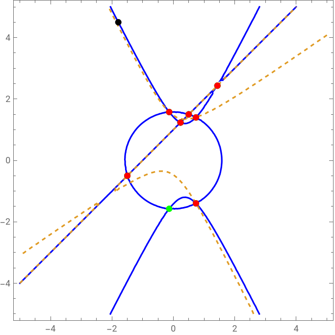
The example pictured above is the polynomial
The two factors are listed in the ordered pair output . The first being
You may wish to normalize by dividing by the smallest coefficient.
This is the hyperbola in the plot above . To get the plot use option plot→m where m is the maximum value you want of x or y.
You may have noticed that this run gives a different result. That is intentional as this is a randomized probabilistic algorithm and may fail on the first attempt. The dashed curves indicate the function h. The red dots are the singular points inside the plotted region used in constructing h. The green dot is a singular point not used, a black dot is a non-singular point used to construct h, this don’t show up with a small value of m. So we see here the intersection of h and the curve fsp is the circle in the center of the plot.
For degree 3, 4 most reducible curves should be factored .
Here no singular points show up on plot . In fact all 4 singular points are complex.
There are several things that can go wrong .
This is usually a fatal error . While complexSingularPoints2D does use random choices it rarely misses affine singular points. This is a rare reducible quartic that fails but that is caused by the fact that some singular points are infinite, not affine. I am not considering this case here.
Here is a somewhat harder example of degree 7
Try again
Note : The two examples are exact and thus can be multiplied by a large number to make them integer coefficient polynomials. Then Mathematica’s Factor can factor them quickly. But singularFactor2D did not know that and this was not the point of this post.
Conclusion
Conclusion
While we cannot give a simple proof why this works, and it may not work on some runs, but it will usually work when we have enough distinct affine singular points. But we do know how this algorithm works. Perhaps this simple heuristic explanation of our theorem will make more sense to more people that a complicated theoretical proof.
Appendix : Code for Functions needed but not described in this paper
Appendix : Code for Functions needed but not described in this paper
This code is explained in my Plane Curve Book, see Appendix A.6, and in my GlobalFunctionsNS.nb on my website. Here is just the code.
CITE THIS NOTEBOOK
CITE THIS NOTEBOOK
A numerical approach to real algebraic curves: number of singular points on a plane algebraic curve
by Barry H Dayton
Wolfram Community, STAFF PICKS, September 19, 2023
https://community.wolfram.com/groups/-/m/t/3015695
by Barry H Dayton
Wolfram Community, STAFF PICKS, September 19, 2023
https://community.wolfram.com/groups/-/m/t/3015695