The Wolfram Emerging Leaders Program: High School (WELP:HS) is a remote, semester-long program designed for exceptional graduates from the Wolfram High School Summer Research Program to continue to develop their skills. Students work in a small group over the course of a semester to do either a research-based project or a product development–based project under the guidance of expert mentors. Projects are centered around a topic at the intersection of the group’s interests.
This essay was written by:
Protein-protein interactions (PPIs) are critical biological processes where two or more proteins bind together to form complexes, enabling diverse cellular functions and signaling pathways. These interactions can be mapped to create a protein interaction network, which provides insights into the underlying biological mechanisms of diseases and cellular processes. In this project, we utilized the Human Protein Atlas database to obtain comprehensive data on over 11,000 proteins and their interactions. By analyzing this extensive dataset, we constructed a detailed PPI network, which may help facilitate a deeper understanding of the functional relationships among proteins in the human body and their role in human health and diseases. We have also used different graph-related analyses to study the roles of important proteins in the network in gene co-expression, pathogenicity, and cancer.
Introduction
Protein-protein interactions (PPIs) are essential biochemical events that occur when two or more proteins physically bind together, forming complexes that enable various cellular processes. These interactions play a crucial role in signal transduction, immune responses, enzymatic activities, and the regulation of gene expression. The specificity and strength of PPIs can influence cellular pathways, making them vital for maintaining cellular homeostasis. Disruptions in these interactions are often implicated in a range of diseases, including cancer, neurodegenerative disorders, and infectious diseases, highlighting their significance in both health and pathology.
Understanding PPIs is fundamental for elucidating cellular mechanisms and developing therapeutic strategies. Protein complex formation can be transient or stable, and the nature of these interactions can vary widely depending on environmental factors and the cellular context. Researchers employ various techniques, such as co-immunoprecipitation, yeast two-hybrid screening, and advanced imaging methods, to study PPIs. Additionally, databases, like the Human Protein Atlas, enable the analysis and visualization of interaction networks, providing valuable insights into the functional roles of proteins and their interdependencies within the cell.
In this project we construct the complete human protein-protein interaction network (PPIN) from information about individual genes, create a function to obtain a network for a protein of specific depth, perform different graph-related analyses on human PPIN, and study the roles of important proteins in the network in gene co-expression, pathogenicity, and cancer.
Human protein-protein interaction network (PPIN) data
The data for individual protein-coding genes is structured as a nested association for efficient access and organization, with the Ensembl ID serving as the primary key. This structured approach ensures that all relevant attributes for each protein, including molecular function, biological processes, and subcellular localization, are easily retrievable. Using the Human Protein Atlas API, we created three primary associations that focus on distinct aspects of the dataset: (1) protein-specific attributes, (2) interaction data for protein-protein connections, and (3) connecting the interactions to broader biological context. This systematic data organization facilitates precise and scalable analyses of the PPI network.
Data for all protein-coding genes forming the human PPIN
Data for all protein-coding genes forming the human PPIN
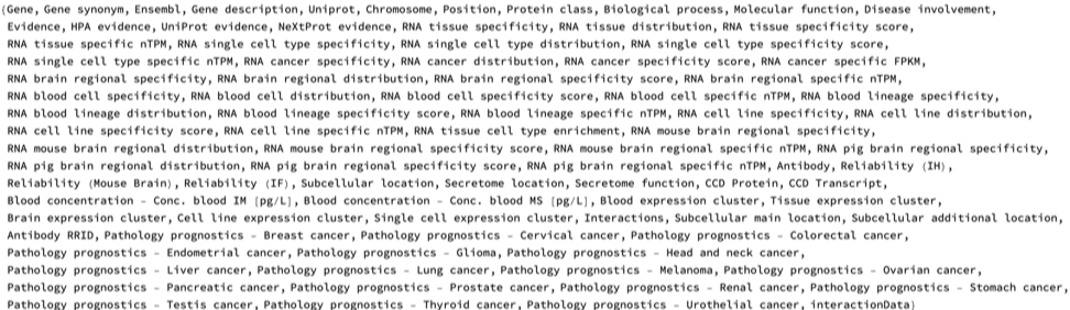
Here is the data for all protein-coding genes involved in human PPIN, sourced from the Wolfram Data Repository. The data is organized by genes' Ensembl IDs and has different attributes like Chromosome, Protein class, Biological process, Molecular function, Disease involvement, etc., with 90 different features:
In[]:=
PPINGeneData=ResourceData["Human Protein Protein Interaction Network Genes"];
In[]:=
Dataset@PPINGeneData

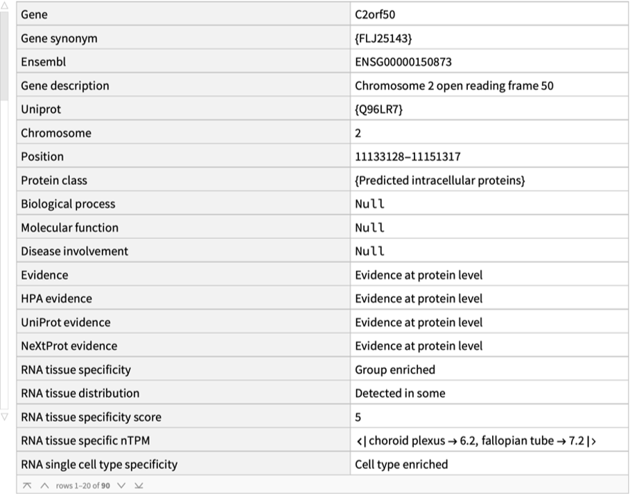
Here is the data for a randomly chosen protein-coding gene:
In[]:=
Dataset@PPINGeneData[Echo@RandomChoice@Keys@PPINGeneData]
»
ENSG00000150873
Out[]=
The number of proteins in the network are:
In[]:=
Length@PPINGeneData
Out[]=
11351
Here are the names of the protein-coding genes corresponding to the proteins that form the PPIN:
In[]:=
PPINGenes=Values@PPINGeneData[[All,"Gene"]];Short@PPINGenes
Out[]//Short=

The keys of the data are the Ensembl IDs of the genes which are its unique identifiers. Since this is standardized and used by the Human Protein Atlas, it is useful to connect the gene names with the Ensembl IDs. Here is an Association of gene names and Ensembl IDs which will be used for computations:
In[]:=
ensemblGeneAssoc=PPINGeneData[[All,"Gene"]];geneEnsemblAssociation=AssociationThread[Values@ensemblGeneAssoc,Keys@ensemblGeneAssoc]

These attributes are included in the data:
In[]:=
Keys@PPINGeneData[[1]]
Out[]=
Protein interaction data
Protein interaction data
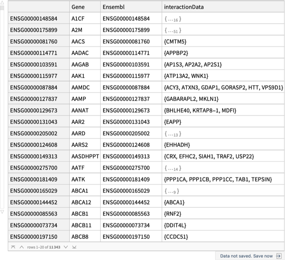
ResourceData["Human Protein Protein Interaction Network Genes", "interactionsOnly"] contains details about the interactions for each protein in the PPIN as provided by the Human Protein Atlas. These interactions describe how proteins communicate with other proteins and function in our body. Each protein is capable of interacting with multiple other proteins. Such interactions can range from direct physical binding to functional associations that contribute to complex biological pathways, emphasizing the interconnected nature of the protein network. This will be used to construct the full PPIN:
In[]:=
interactions=ResourceData["Human Protein Protein Interaction Network Genes","interactionsOnly"];Dataset@interactions
Out[]=
Retrieve the latest version of the data for the protein-coding genes involved in the human PPIN:
Version 24.0 Data
In[]:=
fullDataV24=ResourceData["Human Protein Protein Interaction Network Genes","Version 24.0"];Dataset@fullDataV24

The data used in this essay for further analysis and visualizations is sourced from the first Association, as it contains all data from the Human Protein Atlas version 24.0. The interactions-only data object contains the essential dataset that includes only the protein-coding gene name, Ensembl ID, and interaction data for each gene. This dataset allows for a more directed analysis of the protein-protein interactions relevant to our project.
Protein-Protein Interaction Network Graph
Protein-Protein Interaction Network Graph
Using ResourceData["Human Protein Protein Interaction Network Genes", "interactionsOnly"] we construct the full PPIN, which can be accessed using:
In[]:=
humanPPIN=ResourceData["Human Protein Protein Interaction Network"]
The Human PPIN has 11351 nodes (proteins) and 63088 undirected edges (interactions). We can also obtain different graph measures for all proteins present in the PPIN:
The data is an Association of an Association and we can extract the individual graph measures of a protein in the network:
Visualizations and analysis of proteins in the Human PPIN
The HTT gene, which has the highest connectivity in human PPIN encodes the huntingtin protein, is crucial for brain and nervous system function. While its exact role remains incompletely understood, huntingtin is known to support neuronal development, intracellular transport, and gene expression regulation, particularly by promoting brain-derived neurotrophic factor (BDNF). It also contributes to cell signaling, apoptosis prevention, DNA repair, and immune system regulation. Mutations in the HTT gene, specifically the expansion of CAG trinucleotide repeats, lead to Huntington's disease (HD), a neurodegenerative disorder characterized by motor, cognitive, and emotional impairments. Normal individuals carry 6-35 repeats, while 36 or more repeats are associated with HD risk, with 40 or more guaranteeing disease onset. Mutant huntingtin produces toxic effects, including neuronal damage and immune dysfunction, contributing to the disease's progression.
We can also analyze the genes based on other characteristics, such as the chromosome each of them appears on:
The Human protein-protein interaction network
The project's most valuable insight comes from the comprehensive graph of all interacting proteins in the human body. This graph is constructed by linking nodes—representing proteins in the network—based on their documented interactions in the Human Protein Atlas. This graph is novel to this project and is not readily available in the Human Protein Atlas and will allow users to use Wolfram Language's graph related functionalities for detailed analysis of the human PPIN, some of which are shown in this essay.
The graph serves multiple purposes: it enables the exploration of how proteins influence one another, facilitates targeted analyses of specific proteins and their interaction pathways, and allows for graph-based categorization of proteins using metrics like VertexDegree, BetweennessCentrality, ClosenessCentrality, and shortest path distances. This approach opens doors to understanding complex biological networks and identifying critical players in cellular processes.
The graph serves multiple purposes: it enables the exploration of how proteins influence one another, facilitates targeted analyses of specific proteins and their interaction pathways, and allows for graph-based categorization of proteins using metrics like VertexDegree, BetweennessCentrality, ClosenessCentrality, and shortest path distances. This approach opens doors to understanding complex biological networks and identifying critical players in cellular processes.
As we can see, the full PPIN includes 11351 proteins and includes 63088 interactions.
To visualize the full PPIN, we can use GraphPlot. The names of the protein coding genes are in the Tooltip, which can be seen upon mouse hover when this notebook is downloaded:
The human protein interaction network's structure, consisting of a giant interconnected graph, smaller loops, graphs, and single edges, reflects the complex organization of protein interactions in the cell. The giant interconnected graph represents the core interactome, where most proteins are linked through direct or indirect interactions, enabling widespread communication and coordination of cellular processes. This large component facilitates the flow of information and the propagation of signals across the proteome. Smaller loops and graphs likely represent functional modules or protein complexes that perform specific cellular tasks, allowing for localized and specialized functions. These substructures contribute to the network's modularity, enhancing its robustness and efficiency. Single edges, representing isolated interactions between protein pairs, may indicate transient or condition-specific interactions that are important for fine-tuning cellular responses or adapting to specific environmental cues. This multi-level organization of the protein interaction network enables both global coordination and local specialization, contributing to the overall complexity and adaptability of cellular systems.
Here is the part of the human PPIN of all nodes connecting to 200 largest hubs which are scaled and color coded by their VertexDegree with the protein coding gene names on Tooltip:
◼
Plot
Here is the same plot with the names of the hubs in legends:
The 200 largest hubs of the PPIN forms one giant interconnected network.
Scale-free nature, small-world phenomenon and graph-related analysis of the PPIN
Graph-related analysis and visualizations can reveal key features of the PPIN and highlight the proteins that are most important in the network based on the graph measures.
We can visualize the scale-free nature of the PPIN. A scale-free network is a type of network distinguished by a degree distribution that follows a power law. This implies that the fraction of nodes P(k) with k connections to other nodes is proportional to k^γ, where γ is typically a constant between -2 and -3. The defining feature of such networks is the presence of small number of hubs—nodes with a disproportionately high number of connections—while most nodes have relatively few. This power law distribution results in a long tail, indicating the rarity of highly connected nodes. The formation of these hubs is attributed to preferential attachment, where new nodes are more likely to connect to existing nodes with higher connectivity.
Scale-free networks are prevalent in diverse systems, including social, biological, technological, and information networks. They exhibit unique properties, such as robustness against random failures but susceptibility to targeted attacks on hubs. The topology also influences information flow, often enabling rapid and efficient transmission. Additionally, these networks tend to have high clustering coefficients, forming dense subgraphs linked by hubs, and display the small-world phenomenon, where most nodes are reachable within a few steps. These characteristics provide insights into the behavior and organization of complex systems across various fields.
VertexDegree fraction in the Human PPIN graph, which implies that the human PPIN is a scale free network with a few large hubs:
The human protein-protein interaction network (PPIN) exhibits a scale-free structure, making it particularly interesting to investigate the role of hubs in relation to biological functions, health, and disease. These highly connected nodes may hold key insights into critical processes, including the stability of the network, disease propagation, and potential therapeutic targets.
The scale-free nature of the network can also be analyzed by visualizing the clustering coefficient vs vertex degree plot. In scale-free networks, the log-log plot of mean local clustering coefficient versus vertex degree typically exhibits a distinctive decreasing trend. This relationship is characterized by an inverse correlation between vertex degree and clustering coefficient, often following a power-law decay expressed as C(k) ~ k^(-β), where C(k) is the mean clustering coefficient for vertices of degree k, and β is the decay exponent. This pattern reflects the heterogeneous clustering structure of scale-free networks, where low-degree nodes generally form dense subgraphs or communities with high clustering coefficients, while high-degree nodes (hubs) have lower clustering coefficients as they often serve to connect these dense subgraphs. This behavior is consistent with the hierarchical organization commonly observed in scale-free networks and highlights the crucial role of high-degree nodes in maintaining overall network connectivity.
We can generate a table highlighting the top 25 genes in the human PPIN ranked by VertexDegree, illustrating the behavior of hubs and revealing how a small number of genes exhibit significantly higher interaction levels compared to others:
Here are the importance of the top five hubs in the human PPIN:
◼
The HTT gene codes for the huntingtin protein, which plays crucial roles in various biological functions despite its exact purpose not being fully understood. Huntingtin is essential for normal development before birth and is widely expressed in many tissues, with the highest levels in the brain. Within cells, it is involved in axonal transport, vesicle trafficking, regulation of gene transcription, and protection against apoptosis. The protein also participates in intracellular signaling, DNA repair, and maintenance of epithelial polarity. Mutations in the HTT gene, specifically an expansion of CAG trinucleotide repeats, cause Huntington's disease, a neurodegenerative disorder characterized by progressive psychiatric disruption, cognitive deficits, and loss of motor coordination. Additionally, wild-type huntingtin has been found to regulate human macrophage function, suggesting a role in the immune system.
◼
The CYSRT1 gene codes for the cysteine-rich tail protein 1, which is specifically expressed in cutaneous and oral epithelia. This protein plays a role in the epidermal antimicrobial host defense system. CYSRT1 is found in the upper layers of the suprabasal epidermis, where it colocalizes with late cornified envelope (LCE) proteins. It can interact with members of all LCE groups except LCE6, as demonstrated through yeast two-hybrid screening and coimmunoprecipitation studies. The protein's expression is associated with keratinocyte terminal differentiation and can be induced by disruption of the skin barrier. Importantly, CYSRT1 exhibits antibacterial activity against Pseudomonas aeruginosa, contributing to the skin's constitutive antimicrobial defense. While not directly linked to specific diseases, its role in maintaining skin barrier function and antimicrobial defense suggests that alterations in CYSRT1 could potentially impact skin health and susceptibility to infections.
◼
The GOLGA2 gene encodes the Golgin subfamily A member 2 protein, also known as GM130, which plays crucial roles in maintaining the structure and function of the Golgi apparatus. This protein is involved in the stacking of Golgi cisternae, vesicular transport, and the tethering of transport vesicles to Golgi membranes. GM130 is essential for normal protein transport from the endoplasmic reticulum to the Golgi apparatus and the cell membrane. It also participates in regulating cell adhesion, polarity, and migration. The protein interacts with other Golgi-associated proteins to maintain the integrity of the Golgi complex and facilitate proper vesicle fusion. Mutations in the GOLGA2 gene have been associated with a rare neuromuscular disorder characterized by developmental delay, seizures, progressive microcephaly, and muscular dystrophy. Studies in zebrafish have shown that knockdown of the golga2 gene results in skeletal muscle disorganization and microcephaly, supporting the critical role of this protein in neurodevelopment and muscle function.
◼
The LNX1 gene encodes an E3 ubiquitin ligase that plays diverse roles in neuronal signaling and development. The LNX1 protein contains a RING finger domain and four PDZ domains, allowing it to interact with numerous proteins and regulate their ubiquitination and degradation. In the nervous system, LNX1 is involved in modulating NUMB/NOTCH signaling during cortical neurogenesis, regulating synapse formation and neurotransmission, and controlling the expression and function of the glycine transporter GlyT2. LNX1 also participates in maintaining the structure of the Golgi apparatus and regulating protein transport. While not directly linked to specific diseases, LNX1's role in neuronal signaling suggests it may influence neurodevelopmental processes. Studies have shown that deletion of LNX1 and LNX2 in the central nervous system of mice results in an anxiety-related phenotype, indicating a potential role in mood regulation. Additionally, LNX1's ability to modulate glycinergic neurotransmission through GlyT2 regulation suggests it may influence inhibitory signaling in the central nervous system.
◼
The KRTAP10-8 gene encodes a keratin-associated protein that plays a crucial role in hair formation and structure. This protein is part of the interfilamentous matrix in the hair cortex, where it interacts with hair keratin intermediate filaments. KRTAP10-8 is essential for creating a rigid and resistant hair shaft through extensive disulfide bond cross-linking with the cysteine-rich regions of hair keratins. The protein is classified as a high-sulfur keratin-associated protein, contributing to the matrix that embeds hair keratin filaments. While not directly linked to specific diseases, KRTAP10-8's function in hair structure suggests that alterations in this gene could potentially affect hair quality or growth. Additionally, studies have shown that environmental factors like aflatoxin B1, benzo[a]pyrene, and bisphenol A can affect the expression or methylation of KRTAP10-8, indicating its potential sensitivity to external influences.
The impact of these hubs becomes more evident when we analyze the distances between individual proteins and one of these hubs. In graph theory, the distance between two nodes (or vertices) is defined as the number of edges in the shortest path connecting them. This concept, also known as geodesic distance or shortest-path distance, is fundamental in understanding the structure and properties of graphs. Distance is also essential in algorithms like breadth-first search (BFS) and in computing important graph metrics such as diameter and centrality measures. Understanding distances in graphs is vital for analyzing network efficiency, predicting information spread, and optimizing various network-based systems across diverse fields including computer science, sociology, and biology.
The histogram below illustrates the frequency distribution of the minimum distances from all vertices to their nearest hubs, highlighting the central role of hubs in the network's connectivity.
The histogram below illustrates the frequency distribution of the minimum distances from all vertices to their nearest hubs, highlighting the central role of hubs in the network's connectivity.
We can see that the largest minimum distance from a protein that has a continuous path to to reach a hub is only 6. But most hubs have a GraphDistance of less than 4, signifying very fast information spread from the hubs to all other nodes:
Here is the distances of a protein from the nearest hub:
We can also view a GraphPlot of each vertex whose size if scaled and colored based on the distance to the nearest hub:
We can also visualize the most important proteins based on different centrality measures of the network :
◼
Degree centrality is a fundamental measure of a node's importance in a network, based on the number of direct connections it has. In protein interaction networks, proteins with high degree centrality are often referred to as "hubs" and are considered crucial for maintaining the network's structure and function. These hub proteins typically play essential roles in cellular processes and are more likely to be involved in multiple pathways. High degree centrality in protein networks can indicate proteins that are central to cellular functions, potentially more evolutionarily conserved, and critical for organism survival.
◼
Betweenness centrality measures how often a node acts as a bridge along the shortest path between other nodes in the network. In protein interaction networks, proteins with high betweenness centrality are often called "bottlenecks" and are critical for controlling information flow within the network. These proteins may not necessarily have many direct interactions but play a crucial role in connecting different functional modules or protein complexes. In biological terms, proteins with high betweenness centrality often represent key regulators or mediators in signaling pathways and are potential targets for drug development due to their strategic positions in the network.
◼
Eigenvector centrality assesses a node's importance based not only on its number of connections but also on the importance of the nodes it connects to. In protein interaction networks, proteins with high eigenvector centrality are connected to other highly influential proteins, indicating their involvement in critical cellular processes. This measure can help identify proteins that may not have the highest number of interactions but are connected to other important proteins, potentially revealing hidden key players in biological pathways. Eigenvector centrality can be particularly useful for understanding the propagation of effects through protein networks and identifying proteins that might have significant indirect influences on cellular functions.
Graph Visualization for specific proteins in PPIN
Specifying depth in protein-protein interaction networks (PPINs) strikes a balance between focusing on immediate, highly relevant connections and exploring the broader functional landscape of the network. Shallow depths, such as depth 1, yield a simpler, less dense network that is easier to visualize and analyze both computationally and conceptually. In contrast, deeper networks introduce greater complexity, uncovering additional connections that may be important but can quickly become overwhelming, particularly for highly connected genes.
Depth specification is critical for uncovering biological insights. Certain pathways or processes might only emerge at specific depths; for instance, a protein’s role in a signaling pathway might become apparent only at depth 2 or 3, revealing indirect but functionally significant interactions. By tracing these extended connections, it becomes possible to capture pathway dynamics and prioritize interactions for experimental validation. Direct interactions at depth 1 often represent strong candidates for immediate investigation. In contrast, depth 2 interactions can highlight proteins with indirect but crucial roles in mediating downstream effects. Further exploration at varying depths might reveal conserved interactions or those involved in broader, multi-gene processes.
Indirect connections beyond depth 1 can also provide insights into secondary functions or alternate pathways, which may play critical roles under specific conditions, such as during disease states. Depth-based analysis thus offers a powerful tool for navigating the complexity of PPINs, enabling researchers to target particular interactions for deeper biological exploration.
This function takes a specific protein (given by name of the protein-coding gene) and a specified depth ("NetworkLayers") as input, then generates a graph showing the corresponding connections to the protein. At depth 1, the graph includes the specified protein and all proteins directly interacting with it. A graph of depth 2 expands to include all proteins interacting with those in depth 1, and so on.
The nodes graph can be scaled by different graph measures (e.g., VertexDegree) to highlight important nodes and identify specific interaction hotspots. Additionally, modifying the GraphLayout and VertexLabels allows for custom visualization approaches, making it easier to interpret the network:
Comparing human PPIN and gene co-expression networks in tissues, brain and single cells
Gene co-expression and protein-protein interaction networks
Gene co-expression and protein-protein interaction networks
A gene co-expression network (GCN) is a graph where nodes represent genes, and edges connect genes showing similar expression patterns across multiple locations, samples or conditions. These networks are constructed by calculating expression similarity and applying a significance threshold to determine meaningful relationships. The primary goal is to identify genes that are potentially co-regulated or functionally related based on their coordinated expression profiles.
In contrast, protein-protein interaction (PPI) networks represent physical interactions between protein molecules, with nodes representing proteins and edges indicating direct biochemical contacts. Key differences include the nature of connections (expression similarity vs. physical interactions), level of biological information, and data sources. While GCNs reveal genes with similar expression patterns, PPIs show actual molecular interactions. Both network types are crucial for understanding cellular processes, with GCNs helping identify potential functional gene groups and PPIs providing insights into molecular machinery and signaling pathways.
We can access the gene co-expression networks in the human brain, tissues and different single cell types from ResourceData["Human Protein Atlas"]. In this section, we explore the relationship between PPINs and gene co-expression networks in the human body.
Human PPIN and gene co-expression networks data
Human PPIN and gene co-expression networks data
Data for human PPIN and corresponding graph measures are used from previous sections, the following subsection has details on the GCN data used in this project.
Analysis
Analysis
Relationship between proteins involved in the human PPIN and corresponding protein coding genes in the gene co-expression networks
Relationship between proteins involved in the human PPIN and corresponding protein coding genes in the gene co-expression networks
To find the relationship between proteins involved in the human PPIN and corresponding protein coding genes in the gene co-expression networks we define the Associations for every measure of centrality for the PPIN as well as the gene co-expression networks:
We visualize the LocalClusteringCoefficients of genes common to both the PPIN and tissue-specific gene co-expression networks, with gene names as Tooltips:
The Local Clustering Coefficient (LCC) is a network metric that quantifies how closely a node's neighbors are interconnected, essentially measuring the tendency of nodes to form tightly knit groups. In the context of Protein-Protein Interaction (PPI) networks, a high LCC carries significant biological implications. It often indicates that a protein is part of a functional module or complex, suggesting involvement in specific cellular processes. This property makes LCC a valuable tool for predicting protein functions, identifying important protein complexes, and understanding the modular organization of cellular processes. Furthermore, proteins with high LCC are frequently associated with diseases, making them potential targets for drug development.
High Local Clustering Coefficient (LCC) in gene co-expression networks carries significant biological implications too. It often indicates that genes are part of functional modules or complexes involved in specific cellular processes, with highly clustered genes likely to be functionally related. Networks with high LCC tend to be more robust and resilient to perturbations, maintaining function even when some connections are disrupted. Analyzing LCCs in a network helps researchers infer functions of uncharacterized genes and discover new biological relationships.
High Local Clustering Coefficient (LCC) in gene co-expression networks carries significant biological implications too. It often indicates that genes are part of functional modules or complexes involved in specific cellular processes, with highly clustered genes likely to be functionally related. Networks with high LCC tend to be more robust and resilient to perturbations, maintaining function even when some connections are disrupted. Analyzing LCCs in a network helps researchers infer functions of uncharacterized genes and discover new biological relationships.
Let us visualize the genes that has high LCC values in both PPIN and tissue gene co-expression network:
The size of the protein-coding gene names are scaled by the product of the LCC in the gene co-expression network and PPIN.
◼
Plots for all possible graph measures:
◼
Plot for BetweennessCentrality in PPIN and gene co-expression network in the human brain with gene names in Tooltips:
◼
The correlation values:
As we can see there isn't much correlation between different graph measure pairs. The lack of correlation between graph measures for genes in gene co-expression networks and their corresponding proteins in protein interaction networks can be attributed to several factors:
1. Different biological levels: Gene co-expression networks represent relationships at the mRNA level, while protein interaction networks represent physical interactions at the protein level. These two biological levels can have distinct regulatory mechanisms and dynamics.
2. Temporal and spatial differences: Gene co-expression captures simultaneous expression patterns, which may not directly translate to protein interactions. Proteins can interact even if their corresponding genes are not co-expressed at the same time or in the same cellular compartment.
3. Post-transcriptional regulation: The relationship between mRNA levels and protein abundance is not always linear due to various post-transcriptional regulatory mechanisms, which can affect protein availability for interactions.
4. Network construction methods: Gene co-expression networks are typically built using correlation measures like Pearson correlation, while protein interaction networks are constructed based on experimental evidence of physical interactions. These different approaches can lead to divergent network structures.
5. Interaction dynamics: Protein interactions can be transient or stable, and this dynamic nature may not be captured in gene co-expression data.
6. Functional differences: Co-expressed genes may be involved in similar biological processes without their proteins directly interacting, while interacting proteins may not necessarily be encoded by co-expressed genes.
Understanding these differences is crucial for interpreting and integrating information from both types of networks in systems biology studies in the future. Given the lack of significant correlation between graph measures in the PPIN and co-expression networks, it would be interesting to highlight the most important genes from both networks using a WordCloud visualization:
◼
Here are the WordClouds for different measures where the gene names are scaled and colored by product of the graph measures in the rows for PPIN and in the columns for gene co-expression networks:
We now analyze the scale-free nature of PPIN and gene co-expression networks:
We can see that the scaling exponent is larger for PPIN than for different co-expression networks. Overall the PPINs are much smaller (~60,000 edges) than gene co-expression networks (~3,000,000 edges). The observed differences in the power law exponents and network sizes between the Protein Interaction Network (PIN) and gene co-expression network in humans reflect their distinct biological nature and construction methods.
The larger size of the gene co-expression network indicates that it captures more relationships between genes based on their expression patterns. This is expected as co-expression networks are typically constructed using correlation measures across multiple samples, potentially identifying a broader range of functional relationships. The smaller power law exponent in the co-expression network suggests a more gradual decrease in the frequency of high-degree nodes, implying a relatively higher number of genes with many co-expression partners. This could indicate a more interconnected and less centralized network structure, where groups of genes tend to be co-regulated together. In contrast, the PPIN's higher power law exponent suggests a steeper decline in the frequency of high-degree nodes, pointing to a more centralized network with fewer highly connected hub proteins. These differences underscore the complementary nature of these networks in understanding cellular organization, with co-expression networks capturing broader functional relationships and PPINs representing more specific physical interactions.
The larger size of the gene co-expression network indicates that it captures more relationships between genes based on their expression patterns. This is expected as co-expression networks are typically constructed using correlation measures across multiple samples, potentially identifying a broader range of functional relationships. The smaller power law exponent in the co-expression network suggests a more gradual decrease in the frequency of high-degree nodes, implying a relatively higher number of genes with many co-expression partners. This could indicate a more interconnected and less centralized network structure, where groups of genes tend to be co-regulated together. In contrast, the PPIN's higher power law exponent suggests a steeper decline in the frequency of high-degree nodes, pointing to a more centralized network with fewer highly connected hub proteins. These differences underscore the complementary nature of these networks in understanding cellular organization, with co-expression networks capturing broader functional relationships and PPINs representing more specific physical interactions.
Ordering protein-coding genes by centrality measures
Ordering protein-coding genes by centrality measures
◼
Datasets that contain every centrality measure for each shared gene:
Here we determine the ranking of every gene in every graph/centrality measure pairing:
◼
Dataset:
More detailed research is needed to understand the significance of the proteins and genes with high centrality measures.
Compare human PPIN graph measures for genes and their correlation with average predicted AlphaMissense pathogenicity in proteins
Mutations, AlphaMissense and PPIN
Mutations, AlphaMissense and PPIN
Mutations are changes in the DNA sequence, which can affect the way proteins function in the body. Proteins are made up of chains of amino acids, and the sequence of these amino acids is determined by the genetic code, encoded in RNA transcribed from the DNA. RNA uses codons, three-nucleotide sequences, to specify which amino acid to add during protein synthesis. A single nucleotide change (called a point mutation) alters a codon, potentially changing the resulting amino acid. This can impact protein structure and function, potentially causing diseases like cancer or genetic disorders.
AlphaMissense, developed by Google DeepMind, is an advanced AI model designed to classify missense mutations—mutations where a single amino acid in a protein is replaced by another. Again, such mutations can have a variety of effects on protein function, potentially leading to diseases. AlphaMissense builds on the success of DeepMind’s AlphaFold, utilizing large-scale protein structure and genomic data to predict whether these mutations are likely benign or harmful. Using the model, it predicts the pathogenicity score for any mutation in each amino acid in a protein coded for by a gene in human body.
It can be hypothesized that the pathogenicity potential of mutations might have a correlation with the measures derived from the Human Protein-Protein Interaction Network (PPIN) due to the effects of the interactions involved in functioning of the human body. Thus, the goal of this part is to investigate whether there is any large-scale correlation between the predictions of AlphaMissense and graph measures derived from the Human Protein-Protein Interaction Network (PPIN).
Data to analyze
Data to analyze
In[]:=
PPIN
PPIN
◼
Graph measures for different proteins in the PPIN:
◼
Information about the protein coding genes in the PPIN:
In[]:=
Useful Associations
Useful Associations
◼
AlphaMissense data is organized by Uniprot IDs and these are the Uniprot IDs for which the data is available:
◼
Association of genes in the PPIN and their Uniprot IDs:
Computation steps
Computation steps
AlphaMissense data is organized by Uniprot IDs and can be accessed using the MissenseVariantData function of the Wolfram ProteinVisualization paclet (it might take a while when doing it the first time):
These are the keys for the data:
One of the most important feature of these is "Status". "Status" includes a pathogenicity type for all 19 possible mutations for each amino acid (since there are 20 amino acids in total) in the protein. Thus, it is a list with lists of length 19 for each amino acid. The 19 elements are either "Likely benign," "Ambiguous," or "Likely pathogenic," with these being output based on the "Score" property:
We will also focus on the “MeanPathogenicity,” for our analysis, which is derived from the values in "Score". "MeanPathogenicity" is a value located between 0 (likely benign or harmless) and 1 (likely pathogenic) and is the Mean of 19 pathogenicity "Score" for each amino acid. Let us see their values:
We can see the pathogenicity for all amino acids with the MissenseVariantListPlot function of the ProteinVisualization paclet:
Here, the blue dots and the red dots represent the individual mutations for each amino acid, which are along the x-axis.
Mutations can lead to structural alterations, potentially disrupting binding sites, altering folding stability, impairing functional domains, and more, all of which can influence pathogenic outcomes. Using the MissenseVariantPlot3D function, we can observe the average pathogenicity in the 3D protein structure where each amino acid is colored based on their "MeanPathogenicity" score:
Now, these are the protein-coding genes in human PPIN that we will be focusing on:
For a randomly chosen gene in the PPIN these are the corresponding UniProt IDs:
It is important to note that there can be more than one Uniprot IDs associated with a gene name. However, most have just 1 value.
Thus, we will need to associate each gene in the PPIN to its values obtained from AlphaMissense. So for any given gene in the network we can get a set of mean pathogenicities (one for each amino acid in all proteins connected to a gene):
We can also obtain the pathogenicity status for all of the amino acids for any gene in the PPIN. This is similar to the previous function but returns results in the form of "Likely benign," "Ambiguous," or "Likely pathogenic":
As stated above, there are only three possibilities in the status:
Moving on, for a given gene we can have one of two numbers that can indicate overall pathogenicity:
1. Mean of mean pathogenicity score
2. Fraction of “Likely pathogenic” mutations
1. Mean of mean pathogenicity score
2. Fraction of “Likely pathogenic” mutations
To obtain (1), we need to average out the values obtained in the "MeanPathogenicity" list. This provides us with a single score for each protein.
To obtain (2), we need to first obtain the fractions for Likely benign, Ambiguous, and Likely pathogenic using the values obtained from the pathogenicityStatus function:
We want a single score for each protein, so we should only consider the "Likely pathogenic" fraction. It might be interesting to evaluate "Ambiguous" and "Likely benign" in the future as well.
These single scores for the proteins will be essential for conducting correlation analyses, as they provide a simplified quantitative representation of pathogenicity that can be compared against the other metrics.
Now, we can obtain the different graph measures for any gene in the network and their values for pathogenicity and the fraction mutations with "Likely pathogenic" status:
As mentioned before, the goal of this section is to find if there is any correlation between the following graph measures in human PPIN: ClosenessCentrality, BetweennessCentrality, DegreeCentrality, EigenvectorCentrality, RadialityCentrality, and LocalClusteringCoefficient and pathogenic fraction and average pathogenicity for all genes in the human PPIN for which AlphaMissense data is present.
To do that, we must first generate an association with both the mean pathogenicity and pathogenic fraction values as well as the original six graph measures (This step takes some time because of using pathogenicity and LikelypathogenicFraction function):
Pathogenicity values might not exist for all proteins associated with a gene. So, after filtering out genes without the necessary data, we can now determine the correlation constants between each of the measures. We can first split the association all into lists.
Now, the correlation coefficients between the different measures can be found:
As seen in the grid above, there is not much, if any correlation between the measurements. To see why this is the case, we can plot each of the combinations below:
As seen, there is no obvious linear correlation, and there often seems to be a few clusters where the points are located. However, despite the clustering, slight variation persists across all graphs, suggesting potential underlying complexities in the relationship between the variables, which cannot be understood with just average behaviors.
We can also generate a series of word clouds to visualize and assess the most prevalent proteins across each combination.
Although there was no significant correlations exist between predicted pathogenicity and graph measures in PPIN, more in depth analysis at individual protein level is needed to find relationship between the two.
Compare human PPIN graph measures for genes and their role in different types of cancers
In this section we compare the human protein interaction graph measures with different cancer values to attempt to find any significant correlation between protein interaction networks and cancer survival rates. We also visualize and analyze different plots for mRNA expression and survival in cancer patients in 17 different cancers and the gene's effects on the survival rate of cancer patients.
Cancer Data Visualization
Cancer Data Visualization
We analyzed the distribution and expression of genes in cancers as well as the prognosis on certain types of cancer in relation to a gene expression.
Gene expression data for a given gene in for all cancers:
Gene expression data for a given gene in for all cancers:
This graph shows the mRNA expression for each cancer type and distribution of the expression levels for a specific gene (ITGA5).
Gene expression for a given gene, in a for a group of cancer patients and their survival probability:
Gene expression for a given gene, in a for a group of cancer patients and their survival probability:
Visualize survival vs gene expression levels for ITGA5 in “Renal cancer” in a group of patients:
This graph shows the role of mRNA expression of a certain gene and its effect on the survival rate of a type of cancer over time.
Getting the data for a specific gene for patients diagnosed with a specific cancer:
Using this function we can obtained the detailed survival data for a specific gene and cancer:
In[]:=
This can be applied to all genes and all the different types of cancers to retrieve, visualize, or analyze data. Here is the data for ITGA5 in "Renal cancer" patients:
Visualize the two distributions of mRNA expressions for a given gene for patients with different outcomes for a specific cancer:
Here is the plot for ITGA5 in "Renal Cancer" patients:
This plot shows the difference in the distribution of expression for ITGA5 gene between patients who did(did not) survive with Blue(Red) for Renal cancer and this will help us analyze if there is some effect of this gene on the cancer survival rate.
To find if there is a true difference between the two distributions above and if the gene has some role in "Renal Cancer", we use PearsonChiSquareTest (smaller output value, typically less than 0.05, means the two distributions are likely different with a maximum value of 1 for the exact same distribution). For our analysis we take a really small cut-off of 0.001 to determine effect of gene on cancer prognosis:
Because the P value is <0.05 we know that there is significant difference between gene expressions for ITGA5 in the "Alive" and "Dead" populations from "Renal cancer". We write a small function to extract the above-mentioned P values for a specific gene and cancer:
Not all genes have effects of cancer prognosis. Here is the data for ITGA5 for Breast cancer:
Comparisons of Graph Measures and Cancer Prognosis
Comparisons of Graph Measures and Cancer Prognosis
Here we show an example computation of how to extract correlation between the effect of a gene in a specific cancer to different graph measures for the protein-coding genes in PPIN:
Computation steps for Renal Cancer
Computation steps for Renal Cancer
Here is the Association of protein coding genes and their VertexDegrees in PPIN:
Here are the protein coding genes in PPIN:
We would need to connect the common cancer names to sets of cancer abbreviations by which the source data is organized:
Here are the 17 cancer names used in our analysis:
Here are the different graph measures for the PPIN genes we are interested in:
The names of the genes for which data is available in cancer cancer:
Obtain the genes common to PPIN and a specific cancer:
Obtain the P values for the for each of the common genes in Renal Cancer to analyze its effect on survival:
Obtain the values for a specific graph measure (VertexDegree) for the common genes:
Obtain the correlation between the VertexDegrees and p-values:
Visualize the values for the VertexDegrees and p-values:
As we can see we don't have any significant correlation between VertexDegree of PPIN and p-values of gene expression distribution between "Dead" and "Alive" patients in renal cancer. We will perform the same analysis for all graph measures and 17 different cancers.
All Cancer Types Prognosis and Correlation Calculations
All Cancer Types Prognosis and Correlation Calculations
Here we calculated the p values for all the genes and calculated if those values had any correlation to graph measures in PPIN:
In this array above, each row represents the type of cancer and each column is the correlation value for a graph measure: VertexDegrees, ClosenessCentrality, BetweennessCentrality, DegreeCentrality, EigenvectorCentrality, RadialityCentrality, and LocalClusteringCoefficient. Correlations should be greater then 0.7 for any significant difference or importance.
It appears that EigenvectorCentrality has the largest correlation with P value out of all the different Graphing Values. Many cancers seem to follow a similar pattern for how different graph values correlate with P value, but there are some apparent outliers like Stomach Cancer. Proteins with high eigenvector centrality are connected to other highly connected and influential proteins. This could mean that the expression of highly influential proteins and their interactions with other proteins has a major effect on the mortality rate of Cancer compared to other graph factors.
Conclusion on PPIN Graph Measures Correlations with Different Types of Cancers
Conclusion on PPIN Graph Measures Correlations with Different Types of Cancers
Discussions
In this project we built the whole human protein-protein interaction network (PPIN) using data from the Human Protein Atlas. Detailed graph-related analysis uncovered that human PPIN is a scale-free network. The scale-free nature of human PPIN signifies that a small number of proteins (hubs) have a disproportionately high number of connections, while most proteins have only a few interactions. This structure confers several important properties to the network. It provides stability against random failures, as the majority of proteins have low connectivity, making it unlikely for a hub to be affected by chance. However, this also makes the network vulnerable to targeted attacks on hub proteins, which could significantly disrupt cellular processes. The scale-free topology allows for efficient communication between proteins and contributes to the network's robustness and adaptability. It also reflects the evolutionary complexity of organisms and plays a crucial role in various biological processes, including disease mechanisms and potential drug targets.
We also developed a function to analyze and visualize networks associated with a specific protein. Large scale analysis of the relationship of graph measures of the PPIN with gene co-expression networks, AlphaMissense pathogenicity and mRNA expression in different cancers reveal no significant relationship. This indicates the need for more detailed research at the individual protein and gene level to study these relationships.
We also developed a function to analyze and visualize networks associated with a specific protein. Large scale analysis of the relationship of graph measures of the PPIN with gene co-expression networks, AlphaMissense pathogenicity and mRNA expression in different cancers reveal no significant relationship. This indicates the need for more detailed research at the individual protein and gene level to study these relationships.
Future Directions
Potential future directions may include introducing edge weights based on interaction strength, co-expression levels, and their significance to better capture the essence of the interactions themselves as not all interactions are equal. Dynamic network modeling may also be considered for accounting for context-specific interactions that could be significant.
In future research, exploring the 3D structures of proteins, their functions, and their similarities with protein-protein interaction networks (PPINs) could provide significant insights into the molecular mechanisms underlying cellular processes. By investigating the relationship between protein structure and interaction-network, researchers could identify critical interaction hubs and functional relationships that contribute to network behavior. Understanding how specific structural features influence protein interactions within a PPIN could reveal cellular functions, particularly in the context of a disease. This approach could also reveal how structural motifs drive functional roles, offering new opportunities for targeted drug design and therapy development.
Moreover, integrating 3D structure data with PPINs could help uncover evolutionary relationships among proteins and their functions. Proteins with similar 3D structures may share roles in biological networks, and analyzing these similarities could highlight previously unknown interactions or functions. In the context of a disease, structural changes in proteins, such as mutations or misfolding, could disrupt their normal interactions and contribute to pathological processes. By combining structural data with PPIN analysis, future research could identify such disruptions and reveal disease mechanisms, ultimately leading to novel therapeutic targets.
Use of machine learning (ML) could further enhance these efforts by enabling researchers to analyze large-scale datasets of protein structures, interactions, and functions more effectively. ML algorithms could predict new protein interactions based on structural features or pinpoint critical nodes within PPINs associated with disease. Additionally, ML could improve the accuracy of protein behavior predictions, aiding in the design of targeted therapies. With the advent of advanced technologies such as cryo-electron microscopy and AI-driven tools like AlphaFold, large-scale structural studies could become increasingly feasible, providing rich datasets for ML models to process. In the future, combining 3D structural analysis, PPINs, and machine learning could revolutionize our understanding of biological networks and drive the development of more effective therapeutic strategies.
References
HTT gene:
[1] https://en.wikipedia.org/wiki/Huntingtin
[2] https://pubmed.ncbi.nlm.nih.gov/22180703/
[3] https://medlineplus.gov/download/genetics/gene/htt.pdf
[4] https://www.frontiersin.org/journals/cellular-neuroscience/articles/10.3389/fncel.2021.689332/full
[5] https://pmc.ncbi.nlm.nih.gov/articles/PMC3237673/
[6] https://medlineplus.gov/genetics/gene/htt/
[7] https://www.nature.com/articles/s41598-020-74042-8
[8] https://www.cell.com/neuron/pdf/S0896-6273(16)00096-9.pdf
Human PPIN structure:
[1] https://pmc.ncbi.nlm.nih.gov/articles/PMC4617211/
[2] https://www.nature.com/articles/s41598-022-12201-9
[3] https://academic.oup.com/bioinformatics/article/34/16/2826/4960047?login=false
[4] https://www.frontiersin.org/journals/genetics/articles/10.3389/fgene.2021.635451/full
[5] https://www.nature.com/articles/s41594-022-00910-8
[6] https://academic.oup.com/bioinformatics/article/38/1/125/6366544
[7] https://www.pnas.org/doi/10.1073/pnas.1603992113
[8] https://pmc.ncbi.nlm.nih.gov/articles/PMC5338233/
CYSRT1 gene:
[1] https://pubmed.ncbi.nlm.nih.gov/36804407/
[2] https://patents.google.com/patent/IL295603B2/en
[3] http://irep.ntu.ac.uk/id/eprint/50580/1/Luisa%20Barbato%202022.pdf
[4] https://patentimages.storage.googleapis.com/80/45/35/49e41afda65490/EP4461818A2.pdf
[5] https://www.genecards.org/cgi-bin/carddisp.pl?gene=CYSRT1
[6] https://www.sinobiological.com/resource/cysrt1
[7] https://www.uniprot.org/uniprotkb/A8MQ03/genomic-coordinates
GOLGA2 gene:
[1] https://en.wikipedia.org/wiki/Golgin_subfamily_A_member_2
[2] https://www.bosterbio.com/bosterbio-gene-info-cards/GOLGA2
[3] https://onlinelibrary.wiley.com/doi/abs/10.1111/cge.14053
[4] https://string-db.org/network/homo_sapiens/GOLGA2
[5] https://panelapp.genomicsengland.co.uk/panels/207/gene/GOLGA2/
[6] https://pmc.ncbi.nlm.nih.gov/articles/PMC4975006/
[7] https://cags.org.ae/en/ctga-details/4264/golga2-associated-neurodevelopmental-disorder
[8] https://www.genecards.org/cgi-bin/carddisp.pl?gene=GOLGA2
LNX1 gene:
[1] https://www.frontiersin.org/journals/molecular-neuroscience/articles/10.3389/fnmol.2022.861873/full
[2] https://www.nature.com/articles/s41598-019-51301-x
[3] https://pmc.ncbi.nlm.nih.gov/articles/PMC7373230/
[4] https://www.genecards.org/cgi-bin/carddisp.pl?gene=LNX1
KRTAP10-8 gene:
[1] https://www.genecards.org/cgi-bin/carddisp.pl?gene=KRTAP10-8
[2] https://www.abmgood.com/KRTAP10-8-Adenovirus-Human-26119051.html
[3] https://rgd.mcw.edu/rgdweb/report/gene/main.html?id=RGD%3A1593740
[4] https://cvd.hugeamp.org/gene.html?gene=KRTAP10-8
[5] https://www.proteinatlas.org/ENSG00000187766-KRTAP10-8
[6] https://string-db.org/network/homo_sapiens/KRTAP10-8
[7] https://www.ncbi.nlm.nih.gov/IEB/Research/Acembly/av.cgi?db=human&l=KRTAP10-8
[8] https://www.ncbi.nlm.nih.gov/gene/386681
[9] https://www.sinobiological.com/resource/krtap10-8
[10] https://www.uniprot.org/uniprotkb/P60410/entry
PPIN vs gene co-expression networks:
[1] https://pmc.ncbi.nlm.nih.gov/articles/PMC3333178/
[2] https://bioinformatics.stackexchange.com/questions/13212/difference-between-ppi-networks-and-gene-co-expression-networks
[3] https://en.wikipedia.org/wiki/Gene_co-expression_network
[4] https://academic.oup.com/bioinformatics/article/37/14/1982/6125359?login=false
[5] https://pmc.ncbi.nlm.nih.gov/articles/PMC3896950/
PPIN vs gene co-expression networks scale-free nature:
[1] https://bioinformatics.stackexchange.com/questions/13212/difference-between-ppi-networks-and-gene-co-expression-networks
[2] https://journals.plos.org/plosone/article?id=10.1371%2Fjournal.pone.0240523
[3] https://www.frontiersin.org/journals/genetics/articles/10.3389/fgene.2021.695399/full
[4] https://pmc.ncbi.nlm.nih.gov/articles/PMC5359264/
[5] https://pubmed.ncbi.nlm.nih.gov/34484293/
Acknowledgements
We would like to express our sincere gratitude to Dr. Soutick Saha for his unwavering support, mentorship, and invaluable guidance throughout this project. His insights were instrumental in shaping the direction of our work. We would also like to extend our thanks to the program directors for establishing the framework that made this program possible and for providing us with this incredible opportunity.
CITE THIS NOTEBOOK
CITE THIS NOTEBOOK
Analyzing and visualizing the human protein-protein interaction network
by Wolfram Education Programs
Wolfram Community, STAFF PICKS, February 4, 2025
https://community.wolfram.com/groups/-/m/t/3379945
by Wolfram Education Programs
Wolfram Community, STAFF PICKS, February 4, 2025
https://community.wolfram.com/groups/-/m/t/3379945