This post is largely the result of a conversation I had with Brian Silverman.
Here is the current plot of weekly global COVID-19 deaths:
In[]:=
covidData=ResourceData["Epidemic Data for Novel Coronavirus COVID-19"];
DateListPlot[covidData[Select[FreeQ[#Deaths["Values"],_Missing]&]/*Total/*Differences/*(MovingMap[Total,#,"Week"]&),"Deaths"],FrameLabel"deaths"]
Out[]=
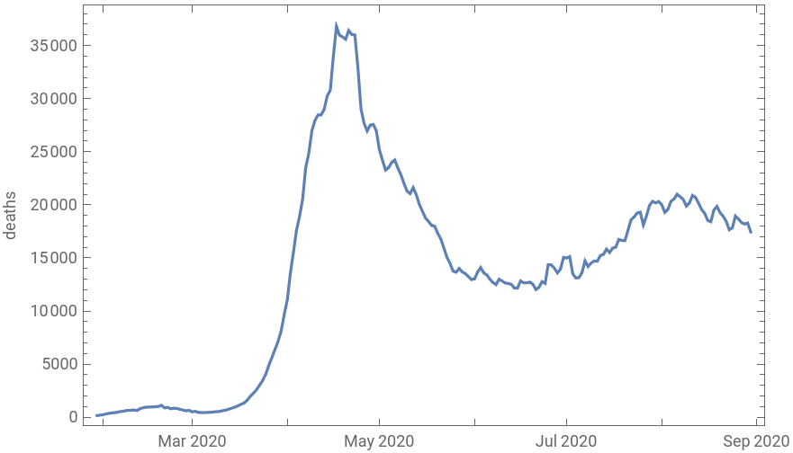
This curve is probably very familiar at this point. It gives the impression that there has been a resurgence in the incidence of COVID, perhaps associated with the lifting of lockdowns. In order to understand what is going on, we start by decomposing this global aggregate into national aggregates, and looking at a small sample:
In[]:=
nationalDeaths=covidData[Query[GroupBy["Country"],Total,"Deaths"]/*Select[GreaterThan[50000]@*Total]/*Map[MovingMap[Total,#,"Week"]&]];
In[]:=
nationalDeathsDerivatives=Differences/@nationalDeaths;
In[]:=
plotCurve[label_,ts_,opts___]:=DateListPlot[ts,PlotLabellabel,PlotRange{All,{0,All}},ImageSize700,AspectRatio1/6,opts]
Column[KeyValueMap[plotCurve,RandomSample[Normal[nationalDeathsDerivatives],5]]]
Out[]=
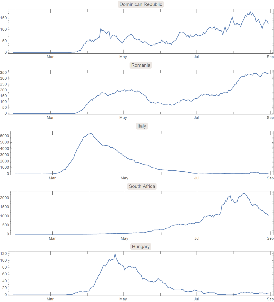
There is a wide variety of behavior here, with some countries primarily showing a peak around April, others showing a peak in August, and some with both. This might suggest that, to an extent, the double peak we see in the global aggregate is not a resurgence of cases in regions lifting lockdowns, but the appearance of COVID in regions which did not experience a peak in May.
In order to visualize this better, we can start by trying to quantify the locations of peaks in these national curves. We could just find the highest point, but this is highly sensitive to outliers and can’t deal with double peaks. It also fails to capture the behavior in the tails, which we can see are also varied (from fat to narrow tails). Instead, think of each peak as a histogram showing the distribution of dates when deaths occurred. The mean or median of this distribution gives us a measure of centrality. We can also look at the standard deviation to get a measure of how “flat” the curve is.
(There are very efficient ways of performing these calculations, but they require more explanation, so I will probably have to write about them in a future post. There isn’t too much data here, so I will use simpler but less efficient methods.)
In[]:=
nationalDists=ProbabilityDistribution[Abs[Interpolation[DeleteMissing[#["Path"],1,2],InterpolationOrder1][x]],{x,#["FirstTime"],#["LastTime"]},Method"Normalize"]&/@Normal[nationalDeathsDerivatives];
nationalMeans=DateObject[N@NExpectation[x,x#]]&/@nationalDists;
nationalStandardDevs=MapThread[UnitConvert[Quantity[N@Sqrt@NExpectation[(x-AbsoluteTime[#2])^2,x#1],"Seconds"],"Days"]&,{nationalDists,nationalMeans}];
In[]:=
nationalMedians=#["Dates"][[FirstPosition[#["Values"],_?(GreaterThan[#["LastValue"]/2])][[1]]]]&/@Normal[nationalDeaths];
The following shows all of the national curves sorted by mean (peak date):
Column[KeyValueMap[plotCurve,KeySortBy[Normal[nationalDeathsDerivatives],nationalMeans]]]
Out[]=

(I don’t know why some of the curves show negative deaths. This is probably some error in the data because I think resurrection on that scale would be more widely reported.)
Apart from a number of data issues, we can see that China had its peak long before anywhere else, and then a procession of countries with well-defined peaks around April. Then there are a few countries that have more erratic curves, and then there are a few with late peaks. Interestingly, there are relatively few which show two proper peaks.
We can also look at how the mean death date varies with geography. Below shows countries with late mean death dates in red, and countries with earlier mean death dates in blue:
(Gray countries had fewer than 50,000 cases and were not counted.)
We can also look at medians:
Finally, we can look at standard deviation. A high standard deviation could be interpreted as the curve being successfully flattened, or it could be interpreted as the outbreak being drawn out for a long time:
US States
US States
We can perform a similar analysis on US states.
The following shows all of the state curves sorted by mean (peak date):
Like with the national curves, most of the high-mortality states either have an early peak or a late peak (California being a notable exception). There are, however, a number of smaller states which show flatter curves, but most of these show lower total mortality, and probably don’t affect the national aggregate curve as much.
Now we can look at how the means vary with geography:
And the medians:
And finally, the standard deviations:
The North East and Midwest both had earlier peaks than in the South or West. The North East had sharp peaks, while the rest of the country had relatively flat peaks.
Conclusion
Conclusion
There are some issues with this kind of analysis, particularly because the weekly deaths curve is clipped at the present, and so statistics like the mean or median can be skewed because we don’t have the whole PDF. However, measures like these still give us a nice way of quantifying many of the properties of the weekly deaths curve that we care about.
We can also see that in most cases the the double peak that appears in aggregates disappears when we look at smaller regions. Finally, we can look at the distribution of national means and medians:
Though both are a bit fuzzy, it does look like there are roughly two peaks: the countries that got COVID in April, and the countries that got COVID in June or August.