Sedimentation in a Newtonian Fluid at Low Reynolds Numbers
Three Spheres vs. a Prolate + a Free Sphere
Authors: Housam Binous and Ahmed Bellagi
Sedimentation in a Newtonian Fluid at Low Reynolds Numbers
Three Spheres vs. a Prolate + a Free Sphere
Authors: Housam Binous and Ahmed Bellagi
Three Spheres vs. a Prolate + a Free Sphere
Authors: Housam Binous and Ahmed Bellagi
Stokesian Dynamics, a method developed by Brady and Bossis in the 80s, simulate the 3D motion of hydrodynamically interacting spheres at low Reynolds numbers . This program was originally written Professor Ron Phillips during his PhD thesis at MIT in 1989. The code was adapted from Fortran 77 to a Mathematica notebook by Housam Binous . Using Euler' s integration scheme was one simplification of the original code that was performed by Housam Binous . The code calls a function NEWTON2, which needs three functions TEMPM, FTMOB and SSI.
This Stokesian Dynamics method was extended to non-Newtonian fluids by Binous and Phillips in 1999 by using FENE dumbbell suspensions.
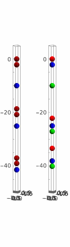
We compare the sedimentation for two cases:
Case 1: a red prolate (formed by gluing two spheres together) and a free blue sphere. In order, to simulate a nonspherical particle (the prolate) , we calculate at each time step a force FC.
Case 2: three spheres (red, blue and green)
Results for both cases are show in the graphics below:
Acknowledgement :
Permission was given by Professor Phillips to post this work in the WEB.
The code uses several functions called NEWTON2, TEMPM, FTMOB and SSI as well as a data.
1/ NEWTON2 computes far-field and adds to it lubrication; it then computes the velocities of the spheres using the mobility matrix and the applied forces.
2/ TEMPM computes far-field mobility.
3/ SSI creates two-body resistance matrix. To do so, it uses interpolation of values given in data as well as analytical expressions. The program then subtracts the two-body far-field mobility from the two-body resistance matrix. The result is the lubrication matrix.
4/ FTMOB creates the two-body far-field mobility.
Case 1: Fall of a prolate (formed by gluing two spheres together) and a free sphere
In[]:=
In[]:=
dt=0.005;
In[]:=
NSPHR=3;NDIM=6 NSPHR;Ng=3 NSPHR;
In[]:=
X[1]=0;Y[1]=0;Z[1]=0;X[2]=0;Y[2]=0;Z[2]=-2.15;X[3]=0;Y[3]=0;Z[3]=-10;
In[]:=
X[1,0]=X[1];Y[1,0]=Y[1];Z[1,0]=Z[1];
X[2,0]=X[2];Y[2,0]=Y[2];Z[2,0]=Z[2];
X[3,0]=X[3];Y[3,0]=Y[3];Z[3,0]=Z[3];
t = 1;
X[2,0]=X[2];Y[2,0]=Y[2];Z[2,0]=Z[2];
X[3,0]=X[3];Y[3,0]=Y[3];Z[3,0]=Z[3];
t = 1;
In[]:=
smallmove[X_,Y_,Z_,t_]:=Module[{UDIFF,Adiff,AFC,FC},For[in=1,in<NSPHR,{For[jn=in+1,jn<NSPHR+1,{DX=X[[jn]]-X[[in]];DY=Y[[jn]]-Y[[in]];DZ=Z[[jn]]-Z[[in]];DR=Sqrt[DX^2+DY^2+DZ^2];jn++}];in++}];While[DR<2,{X[[1]]=X[[1]]+0.004*DX;X[[2]]=X[[2]]-0.004*DX;Y[[1]]=Y[[1]]+0.004*DY;Y[[2]]=Y[[2]]-0.004*DY;Z[[1]]=Z[[1]]+0.004*DZ;Z[[2]]=Z[[2]]-0.004*DZ;For[in=1,in<NSPHR,{For[jn=in+1,jn<NSPHR+1,{DX=X[[jn]]-X[[in]];DY=Y[[jn]]-Y[[in]];DZ=Z[[jn]]-Z[[in]];DR=Sqrt[DX^2+DY^2+DZ^2];jn++}];in++}];}];FU={0,0,-4,0,0,-4,0,0,-4,0,0,0,0,0,0,0,0,0};NEWTON2[X,Y,Z,FU,t];For[i=1,i<4,{UDIFF[i]=UNEW[i+3]-UNEW[i];i++}];Adiff=Table[0,{i,1,3},{i,1,3}];For[in=1,in<4,{For[jn=1,jn<4,Adiff[[in,jn]]=Amm[[in,jn]]-Amm[[in,jn+3]];jn++];in++}];AFC=Inverse[Adiff];For[i=1,i<4,{FC[i]=0;i++}];For[in=1,in<4,{For[jn=1,jn<4,FC[in]=FC[in]+0.5AFC[[in,jn]]UDIFF[jn];jn++],in++}];For[in=1,in<4,{FU[[in]]=FU[[in]]+FC[in];FU[[in+3]]=FU[[in+3]]-FC[in];in++}];NEWTON2[X,Y,Z,FU,t];If[t==1019,Print[Table[FC[i],{i,1,3}]," ",Table[FU[[i]],{i,1,6}]]];]
In[]:=
For[t=1,t<1020,{smallmove[{X[1,t-1],X[2,t-1],X[3,t-1]},
{Y[1,t-1],Y[2,t-1],Y[3,t-1]},{Z[1,t-1],Z[2,t-1],Z[3,t-1]},t];
X[1,t]=X[1,t-1]+UNEW[1]*dt;Y[1,t]=Y[1,t-1]+UNEW[2]*dt;Z[1,t]=Z[1,t-1]+UNEW[3]*dt;
X[2,t]=X[2,t-1]+UNEW[4]*dt;Y[2,t]=Y[2,t-1]+UNEW[5]*dt;Z[2,t]=Z[2,t-1]+UNEW[6]*dt;
X[3,t]=X[3,t-1]+UNEW[7]*dt;Y[3,t]=Y[3,t-1]+UNEW[8]*dt;Z[3,t]=Z[3,t-1]+UNEW[9]*dt;
t++}]
{0.,0.,-11.2721} {0.,0.,-15.2721,0.,0.,7.27211}
Initially the prolate (the doublet show in red) catches up with the blue sphere.
Then, the blue sphere and red prolate fall together as a triplet
Then, the blue sphere and red prolate fall together as a triplet
In[]:=
S1=Show[Graphics3D[{{Darker@Red,Sphere[{X[1,539],Y[1,539],Z[1,539]},0.99995]},{Darker@Red,Sphere[{X[2,539],Y[2,539],Z[2,539]},0.99995]},{RGBColor[0,0,1],Sphere[{X[3,539],Y[3,539],Z[3,539]},0.99995]}}],Graphics3D[{{Darker@Red,Sphere[{X[1,1019],Y[1,1019],Z[1,1019]},0.99995]},{Darker@Red,Sphere[{X[2,1019],Y[2,1019],Z[2,1019]},0.99995]},{RGBColor[0,0,1],Sphere[{X[3,1019],Y[3,1019],Z[3,1019]},0.99995]}}],Graphics3D[{{Darker@Red,Sphere[{X[1],Y[1],Z[1]},0.99995]},{Darker@Red,Sphere[{X[2],Y[2],Z[2]},0.99995]},{RGBColor[0,0,1],Sphere[{X[3],Y[3],Z[3]},0.99995]}}],Axes->True]
Out[]=

Case 2: Fall of three sphere
In[]:=
smallmove2[X_,Y_,Z_,t_]:=Module[{UDIFF,Adiff,AFC,FC},For[in=1,in<NSPHR,{For[jn=in+1,jn<NSPHR+1,{DX=X[[jn]]-X[[in]];DY=Y[[jn]]-Y[[in]];DZ=Z[[jn]]-Z[[in]];DR=Sqrt[DX^2+DY^2+DZ^2];jn++}];in++}];While[DR<2,{X[[1]]=X[[1]]+0.004*DX;X[[2]]=X[[2]]-0.004*DX;Y[[1]]=Y[[1]]+0.004*DY;Y[[2]]=Y[[2]]-0.004*DY;Z[[1]]=Z[[1]]+0.004*DZ;Z[[2]]=Z[[2]]-0.004*DZ;For[in=1,in<NSPHR,{For[jn=in+1,jn<NSPHR+1,{DX=X[[jn]]-X[[in]];DY=Y[[jn]]-Y[[in]];DZ=Z[[jn]]-Z[[in]];DR=Sqrt[DX^2+DY^2+DZ^2];jn++}];in++}];}];FU={0,0,-1.25,0,0,-1.25,0,0,-1.25,0,0,0,0,0,0,0,0,0};NEWTON2[X,Y,Z,FU,t];]
In[]:=
dt=0.005;
In[]:=
For[t=1,t<2850,{smallmove2[{X[1,t-1],X[2,t-1],X[3,t-1]},
{Y[1,t-1],Y[2,t-1],Y[3,t-1]},{Z[1,t-1],Z[2,t-1],Z[3,t-1]},t];
X[1,t]=X[1,t-1]+UNEW[1]*dt;Y[1,t]=Y[1,t-1]+UNEW[2]*dt;Z[1,t]=Z[1,t-1]+UNEW[3]*dt;
X[2,t]=X[2,t-1]+UNEW[4]*dt;Y[2,t]=Y[2,t-1]+UNEW[5]*dt;Z[2,t]=Z[2,t-1]+UNEW[6]*dt;
X[3,t]=X[3,t-1]+UNEW[7]*dt;Y[3,t]=Y[3,t-1]+UNEW[8]*dt;Z[3,t]=Z[3,t-1]+UNEW[9]*dt;
t++}]
Initially, the blue and red sphere catch up with the green sphere.
Then, the blue and green spheres fall as a doublet while the red sphere lags behind
Then, the blue and green spheres fall as a doublet while the red sphere lags behind
In[]:=
S2=Show[Graphics3D[{{RGBColor[1,0,0],Sphere[{X[1,2745],Y[1,2745],Z[1,2745]},0.99995]},{RGBColor[0,0,1],Sphere[{X[2,2745],Y[2,2745],Z[2,2745]},0.99995]},{RGBColor[0,1,0],Sphere[{X[3,2745],Y[3,2745],Z[3,2745]},0.99995]}}],Graphics3D[{{RGBColor[1,0,0],Sphere[{X[1,1145],Y[1,1145],Z[1,1599]},0.99995]},{RGBColor[0,0,1],Sphere[{X[2,1145],Y[2,1145],Z[2,1599]},0.99995]},{RGBColor[0,1,0],Sphere[{X[3,1145],Y[3,1145],Z[3,1599]},0.99995]}}],Graphics3D[{{RGBColor[1,0,0],Sphere[{X[1],Y[1],Z[1]},0.99995]},{RGBColor[0,0,1],Sphere[{X[2],Y[2],Z[2]},0.99995]},{RGBColor[0,1,0],Sphere[{X[3],Y[3],Z[3]},0.99995]}}],Axes->True]
Out[]=

Visual comparison of cases 1 and 2