We develop a general framework for Monte Carlo Tree Search (MCTS) on two-player board games and evaluate its efficacy by conducting comparative analysis on the use of varying time constraints, selection functions, and simulation models.
Introduction
Introduction
In 2016, the world saw a historic moment in the field of AI when AlphaGo, a program developed by Google DeepMind, defeated the human world champion in the game of Go. This achievement was made possible not only by advancements in artificial neural network and reinforcement learning techniques, but also the Monte Carlo Tree Search (MCTS), which serves as the backbone of AlphaGo. MCTS is a tree search algorithm that combines Markov decision processes with reinforcement learning, allowing it to explore large solution spaces and find optimal solutions. When paired with neural networks, which can learn to evaluate positions and predict outcomes, MCTS becomes an unstoppable force in games like Go, Chess, and Poker. But MCTS is not limited to games; its applications extend to fields like finance, logistics, and even scientific research, wherever complex decision-making and planning are required.
The recent proliferation of large language models (LLMs) and other machine learning techniques has launched the field of artificial intelligence to unprecedented heights. Nevertheless, despite these advances, the holy grail of general problem-solving and planning remains unsolved. The development of algorithms that can reason, plan, and make decisions in complex, dynamic environments continues to pose a significant challenge. In this context, search algorithms like MCTS have emerged as a promising candidate, with some experts positing that their application could unlock general problem-solving. As we continue to advance AI research, a nuanced understanding of MCTS and its various implementations becomes increasingly imperative.
To comprehensively evaluate the efficacy of MCTS, we have developed a general framework that can accommodate a wide range of MCTS algorithms, including neural network based ones. Our modular approach allows us to seamlessly integrate our MCTS implementation with many games and domains, facilitating a comparative analysis of different algorithms. Furthermore, we have created simulation functions that allow us to benchmark the performance of our MCTS implementation against existing algorithms like minimax, while also conducting mathematical validation to ensure its accuracy. To optimize the testing process, we have selected Tic-Tac-Toe as a baseline game, providing a simple yet effective way to evaluate the strengths and weaknesses of different MCTS strategies. By using this approach, we aim to distill the essential characteristics of effective MCTS implementations and provide a foundation for further research and development of MCTS in Wolfram Language.
The recent proliferation of large language models (LLMs) and other machine learning techniques has launched the field of artificial intelligence to unprecedented heights. Nevertheless, despite these advances, the holy grail of general problem-solving and planning remains unsolved. The development of algorithms that can reason, plan, and make decisions in complex, dynamic environments continues to pose a significant challenge. In this context, search algorithms like MCTS have emerged as a promising candidate, with some experts positing that their application could unlock general problem-solving. As we continue to advance AI research, a nuanced understanding of MCTS and its various implementations becomes increasingly imperative.
To comprehensively evaluate the efficacy of MCTS, we have developed a general framework that can accommodate a wide range of MCTS algorithms, including neural network based ones. Our modular approach allows us to seamlessly integrate our MCTS implementation with many games and domains, facilitating a comparative analysis of different algorithms. Furthermore, we have created simulation functions that allow us to benchmark the performance of our MCTS implementation against existing algorithms like minimax, while also conducting mathematical validation to ensure its accuracy. To optimize the testing process, we have selected Tic-Tac-Toe as a baseline game, providing a simple yet effective way to evaluate the strengths and weaknesses of different MCTS strategies. By using this approach, we aim to distill the essential characteristics of effective MCTS implementations and provide a foundation for further research and development of MCTS in Wolfram Language.
What is MCTS?
What is MCTS?
Monte Carlo Tree Search (MCTS) is a heuristic search algorithm that combines the principles of Monte Carlo sampling with tree-based search strategies. It is designed to navigate large state spaces efficiently by selectively exploring promising paths while maintaining a balance between exploration and exploitation. MCTS constructs a search tree incrementally, where each node represents a state in the problem domain, and edges represent transitions between states. The algorithm iteratively builds this tree by simulating possible future scenarios and using the results to guide further exploration, ultimately converging on optimal or near-optimal solutions.
The MCTS algorithm operates on the fundamental tension between exploration and exploitation, a common paradigm in reinforcement learning and decision-making under uncertainty. Exploration involves investigating new, potentially promising areas of the search space, while exploitation focuses on using known information to make optimal decisions. MCTS addresses this trade-off through its four primary phases: Selection, Expansion, Simulation, and Backpropagation. These phases work in concert to build and refine the search tree, as discussed in the section below.
Our implementation of MCTS uses a state-centric approach, eschewing explicit action representation in favor of direct state-to-state transitions. This design choice simplifies the algorithm’s structure and enhances its flexibility across various problem domains. Each node in our tree encapsulates three key attributes: a score value, representing the node’s estimated quality; a visit count, tracking the frequency of node traversal; and a prior probability, which can be utilized to incorporate domain-specific knowledge or heuristics. The tree structure itself is represented as a Wolfram Language Graph object, facilitating efficient traversal and manipulation.
The MCTS algorithm operates on the fundamental tension between exploration and exploitation, a common paradigm in reinforcement learning and decision-making under uncertainty. Exploration involves investigating new, potentially promising areas of the search space, while exploitation focuses on using known information to make optimal decisions. MCTS addresses this trade-off through its four primary phases: Selection, Expansion, Simulation, and Backpropagation. These phases work in concert to build and refine the search tree, as discussed in the section below.
Our implementation of MCTS uses a state-centric approach, eschewing explicit action representation in favor of direct state-to-state transitions. This design choice simplifies the algorithm’s structure and enhances its flexibility across various problem domains. Each node in our tree encapsulates three key attributes: a score value, representing the node’s estimated quality; a visit count, tracking the frequency of node traversal; and a prior probability, which can be utilized to incorporate domain-specific knowledge or heuristics. The tree structure itself is represented as a Wolfram Language Graph object, facilitating efficient traversal and manipulation.
The Four Phases
The Four Phases
In[]:=
Grid{Text[Style["Selection",Large,Bold,Darker[Red]]],Text[Style["Expansion",Large,Bold,Darker[Red]]],Text[Style["Simulation",Large,Bold,Darker[Red]]],Text[Style["Backpropagation",Large,Bold,Darker[Red]]]},
,
,
,
,Frame->{All,False},Spacings->{1,0.5}
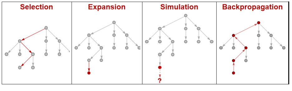
Selection
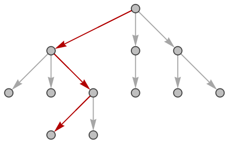
Selection
Out[]=
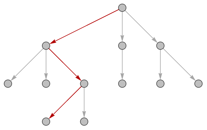
The Selection phase is a critical component of the Monte Carlo Tree Search algorithm, responsible for traversing the existing search tree from the root node to either a leaf node or an unexpanded node. This process is guided by a selection policy that balances exploration of less-visited nodes with exploitation of nodes that have shown promise in previous iterations.The traversal begins at the root node and recursively selects child nodes until reaching a termination condition. At each step, the selection policy evaluates all child nodes of the current node and chooses the most promising one based on a specified criterion. This criterion is typically embodied in an Upper Confidence Bound (UCB) function, which assigns a value to each node that combines its estimated value with an exploration term.The value of a node in MCTS is a statistical estimate of the expected outcome from that node, based on previous simulations. This value is typically represented as a win rate or an average score, depending on the domain. The exploration term encourages the algorithm to visit less-explored nodes, ensuring a comprehensive search of the state space.Several UCB functions have been proposed in the literature, each with its own characteristics and trade-offs. The most common is the UCT (Upper Confidence Bounds for Trees) function:Where is the estimated value of taking action in state , is the number of times the parent state has been visited, is the number of times action a has been taken in state , and is an exploration constant.An alternative formulation is PUCT (Predictor + UCT), which incorporates prior probabilities:Where is the prior probability of selecting action in state , often derived from domain knowledge or learned models.Our implementation provides users with a choice of predefined UCB functions, including UCT and PUCT. Additionally, we offer the flexibility to define custom UCB functions, selection policies, and value functions. This allows for domain-specific optimizations and experimentation with novel selection strategies.
UCT(s,a)Q(s,a)+c
lnN(s)
N(s,a)
Q(s,a)
a
s
N(s)
s
N(s,a)
s
c
PUCT(s,a)Q(s,a)+c·P(s,a)·
N(s)
1+N(s,a)
P(s,a)
a
s
Expansion
Expansion
Out[]=
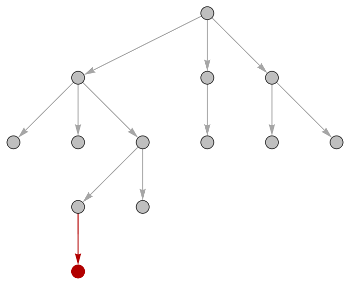
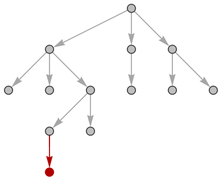
The Expansion phase is responsible for growing the search tree by adding one or more child nodes to a selected leaf node. This process occurs when the Selection phase reaches a node that has not been fully expanded, i.e., a node for which not all possible child states have been added to the tree.
The expansion process typically involves generating all possible legal moves from the current state and creating corresponding child nodes. However, in domains with large branching factors, it may be more efficient to add only a subset of children at each expansion step.
Prior probabilities play an important role in the Expansion phase by influencing the order in which nodes are added to the tree and explored. These priors can be derived from various sources, including domain-specific heuristics, pattern databases, or machine learning models. By prioritizing the expansion of more promising nodes, the algorithm can focus its computational resources on the most relevant parts of the search space.
Our implementation provides a flexible framework for defining prior probability functions. Users can specify custom functions that assign probabilities to potential moves based on any desired criteria. These functions can range from simple heuristics to sophisticated machine learning models, such as neural networks trained on expert gameplay data.
The expansion process typically involves generating all possible legal moves from the current state and creating corresponding child nodes. However, in domains with large branching factors, it may be more efficient to add only a subset of children at each expansion step.
Prior probabilities play an important role in the Expansion phase by influencing the order in which nodes are added to the tree and explored. These priors can be derived from various sources, including domain-specific heuristics, pattern databases, or machine learning models. By prioritizing the expansion of more promising nodes, the algorithm can focus its computational resources on the most relevant parts of the search space.
Our implementation provides a flexible framework for defining prior probability functions. Users can specify custom functions that assign probabilities to potential moves based on any desired criteria. These functions can range from simple heuristics to sophisticated machine learning models, such as neural networks trained on expert gameplay data.
Simulation
Simulation
Out[]=
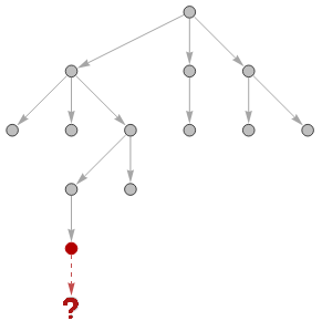
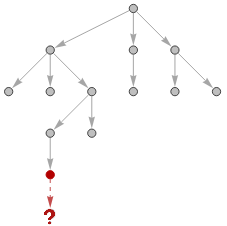
The Simulation phase, also known as the rollout or playout phase, is responsible for estimating the value of newly expanded nodes. This estimation is crucial for guiding the search process and updating the statistics of nodes in the tree. The value of a node in MCTS represents an estimate of the expected outcome from that node. This value is typically expressed as a win rate for games with binary outcomes, or as an expected score for games with more complex scoring systems.
The traditional approach to simulation is the random rollout. Starting from the state represented by the newly expanded node, the algorithm simulates a sequence of random moves until reaching a terminal state. The outcome of this terminal state is then used as the value estimate for the node. The time complexity of a single rollout is linear with respect to the game length, as it involves simulating a complete game from the current state to termination.
To improve the accuracy of value estimates, multiple rollouts can be performed for each node (multi-rollout approach). The final value estimate is then computed as the average outcome across all rollouts. While this approach can provide more reliable estimates, it comes at the cost of increased computational complexity.
An alternative to random rollouts is the use of neural network-based value functions. In this approach, a trained neural network directly predicts the expected outcome of a given state, without the need for explicit simulation. This method can be particularly effective in domains where high-quality training data is available and can significantly reduce the computational cost of the Simulation phase.
Our implementation allows users to provide custom rollout functions, enabling flexibility in the simulation strategy. This can include traditional random rollouts, policy-guided rollouts, multi-rollout approaches, or neural network-based value estimators.
The traditional approach to simulation is the random rollout. Starting from the state represented by the newly expanded node, the algorithm simulates a sequence of random moves until reaching a terminal state. The outcome of this terminal state is then used as the value estimate for the node. The time complexity of a single rollout is linear with respect to the game length, as it involves simulating a complete game from the current state to termination.
To improve the accuracy of value estimates, multiple rollouts can be performed for each node (multi-rollout approach). The final value estimate is then computed as the average outcome across all rollouts. While this approach can provide more reliable estimates, it comes at the cost of increased computational complexity.
An alternative to random rollouts is the use of neural network-based value functions. In this approach, a trained neural network directly predicts the expected outcome of a given state, without the need for explicit simulation. This method can be particularly effective in domains where high-quality training data is available and can significantly reduce the computational cost of the Simulation phase.
Our implementation allows users to provide custom rollout functions, enabling flexibility in the simulation strategy. This can include traditional random rollouts, policy-guided rollouts, multi-rollout approaches, or neural network-based value estimators.
Backpropagation
Backpropagation
Out[]=
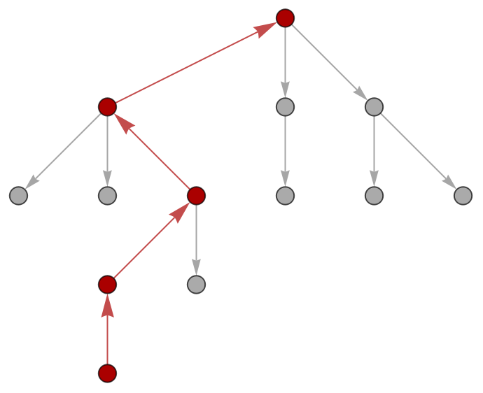
Implementation
Implementation
The following section will break down the elements of our final MonteCarloTreeSearch code and clarify elements of its usage. For demonstration purposes, we will use a 3x3 Tic-Tac-Toe game — chosen for its small state space and simple game mechanics.
First, we must understand how data is represented inside MonteCarloTreeSearch:
State-Based Approach
State-Based Approach
Unlike some other MCTS implementations, we use a state-only approach without actions for each node. This allows for simpler usage.
◼
Game states must be paired with their associated player for proper backpropagation.
◼
We use an association with “Player” as a monotonic value and “State” as any expression.
In the this Tic-Tac-Toe state, “Player” refers to the player that made the last move on the current board and alternates between 1 (X) and -1 (O). “State” encodes the game board containing all the moves that have been made. Methods for displaying the game are kept separate from the data stored in the state association.
Monte Carlo Tree Representation
Monte Carlo Tree Representation
We boiled down what’s needed for a Monte Carlo Tree into five key components, stored as an association:
This association representation of an MCTS tree is used extensively across our functions. Users can easily access any of the data above using their respective keys.
For example, what is the best opening move in tic-tac-toe?
MonteCarloTreeSearch can also begin at any point in the middle of a game, such as given the following state:
The obvious move is for O to block, and MonteCarloTreeSearch agrees.
Arguments
Arguments
MonteCarloTreeSearch accepts four arguments: an initial game state or initial Monte Carlo Tree, an iterator, a rollout function, and the number of iterations the algorithm should run. One “iteration” of MonteCarloTreeSearch means it undergoes each of the four phases (Selection, Simulation, Expansion, Backpropagation) once.
Iterators
Iterators
An “iterator” function should accept a state as an input and return a list of all possible next states.
This Tic-Tac-Toe iterator was given an empty board as input and returned all valid opening moves as output. If the game has ended, iterator should give an empty list.
Note that it is up to the user to define which next states are acceptable. Our Tic-Tac-Toe iterator does not “canonicalize” (categorize rotational and reflectional symmetries as equivalent and choose one to be default) out of convenience for lookup processes in MonteCarloTreeSearch, though possible.
Rollout
Rollout
Rollout is another function the user supplies to MonteCarloTreeSearch, and should evaluate the expected winner for a given game state. This information is later used to update node values in the Backpropagation phase. One potential method is making random moves on a given board until a winner is determined.
Visualization of a random rollout of a tic-tac-toe game
For accessibility, we have also included the code for a default rollout function — provided the user has created an iterator (see previous section) and a winner function (accepts a state as input and returns the winner). Note that it is assumed in that the winner function returns 0 for ties and values that match the name of the “Player” key of the game state for wins. Our rollout also takes an optional 3rd argument that causes the function to average the results of n rollouts, which will be discussed in detail later.
MonteCarloTreeSearch Definition
MonteCarloTreeSearch Definition
Now that we have some basic intuition on MonteCarloTreeSearch usage, we can break down the actual code behind the algorithm.
IterateMonteCarlo is a helper function for MonteCarloTreeSearch that takes in a current node and all the information for the current Monte Carlo Tree. Based on that information, it chooses one of the four phases to complete next and returns a new Monte Carlo Tree. The overall MonteCarloTreeSearch function operates by repeatedly calling IterateMonteCarlo until the iteration or time limit is reached.
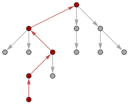
BackPropagate is helper function that completes the Backpropagation phase when called, updating the scores and visits of all nodes in the path from the current to the root based on information from the rollout.
MonteCarloTreeSearch is overloaded depending on the initial condition given. If given an initial state/single node, MonteCarloTreeSearch computes a new game tree from scratch. MonteCarloTreeSearch alternatively accepts a Monte Carlo Tree (the output of a previous MonteCarloTreeSearch) as the initial argument and builds upon the existing data. Supplying the results of a previous MonteCarloTreeSearch reduces the necessary number of iterations to produce reasonable results for a next move.
bestMove is a helper function for the “NextMove” key of MonteCarloTreeSearch. It accepts a Monte Carlo Tree and current state, computing the next state after current that has the highest value.
Optional Arguments
Optional Arguments
MonteCarloTreeSearch accepts various optional arguments, discussed in detail below:
UCB Function
UCB Function
During the Selection phase, the next nodes in the MCTS tree to visit are determined by the highest score returned from a UCB function. Different UCB functions balance between node values and exploration strategies differently.
Typically, UCB scores are higher for nodes with:
◼
High estimated value
◼
Low visit count
◼
High parent visit count
The following association encodes four commonly used UCB functions:
MonteCarloTreeSearch will default to UCB1 if the option is not specified. Users can choose to use a different UCB function from the choices shown above by specifying “UCBFunction” -> Key as an additional argument, or encode a custom UCBFunction entirely and specify “UCBFunction” -> FunctionName. Any custom UCB function defined by the user must still have the following arguments: score of current node, number of times it has been visited, number of times its parent has been visited, a probability value given by the prior function (covered in detail later, but can default to 1), and an exploration constant c.
Exploration Constant
Exploration Constant
The exploration constant is an argument to the UCB function that helps give bias towards less-visited nodes over those with higher values. Users can specify “ExplorationConstant” -> c where c is a positive, real number. Otherwise, the exploration constant defaults to 2.
Value Function
Value Function
Each node in the graph has a value that indicates its expected return, or how good of a next move it would be. By default, the value of a node is score/visits — in the context of games, this can be thought of as the node’s “win rate” after many simulations. Users may specify a custom value function by giving MonteCarloTreeSearch the extra argument “ValueFunction” -> FunctionName.
Selection Function
Selection Function
A selection function can optionally replace the UCB function and Value function to otherwise determine how the Monte Carlo Tree should be traversed. The function should accept the entire Monte Carlo Tree association and a current node as input and return one of the children of the current node to go to. Users can specify a custom selection function by using the syntax “SelectionFunction” -> FunctionName as an extra argument. Note that custom selection functions are mutually exclusive with UCB and Value functions, meaning that if you specify all three, the UCBFunction and ValueFunction will do nothing.
Prior Function
Prior Function
Prior functions are a way of initializing newly added nodes with probabilities to influence the algorithm’s decisions regarding its future reward before going through the process of many simulations. By default, the “prior” value assessment of every node is 1. Custom-defined prior functions should accept a state and output a real number that indicates its probability of a good return. Users can specify a custom prior function to MonteCarloTreeSearch by giving the argument “PriorFunction” -> FunctionName.
Prior functions can help MCTS result in convergence after fewer iterations. In the context of many games, the state space is small enough that simple heuristics, lookup tables, or even neural networks can be used as a shortcut to determining the viability of a certain move.
TimeGoal
TimeGoal
MonteCarloTreeSearch always accepts a natural number n as the number of maximum iterations it should complete before returning its result. However, MCTS is more often constrained by time requirements than iterations. In applications such as computer chess or computer Go, there is a time limit for the algorithm to make a move. Thus when the option TimeGoal is set, the algorithm terminates when it has run for the specified number of seconds or undergone the maximum iterations, whichever comes first.
By default, TimeGoal is set to Infinity:
Users may set an alternative time limit by giving the argument TimeGoal -> seconds, so that the algorithm terminates even before hitting 150 iterations.
Analysis
Analysis
In the following section, we aim to establish more intuition into how users can utilize our MCTS algorithm and demonstrate how toggling the various parameters changes MCTS’s effectiveness.
To objectively quantify how well MCTS performs, we will compare how MCTS plays tic-tac-toe with how the algorithm minimax plays, as minimax finds perfect solutions by analyzing a complete game graph to guarantee either a win or a tie.
Multi Rollout
Multi Rollout
The value returned by a single rollout alone is somewhat arbitrary. One way to improve this process is averaging multiple rollouts in order to get a more accurate assessment of a node’s future reward. We can run MonteCarloTreeSearch using both rollout and multi-rollout on the same initial board to compare their results:
Nodes are colored on a spectrum of red (lowest win-rate) to green (highest win-rate). Hover over nodes to display their game boards.
Using multiple rollout with n = 10 (top row) results in more nuanced information and less variance than the singular version across runs (bottom row). This may result in convergence in fewer iterations, though because rollout can be a computationally intensive process, the benefits from preforming rollout multiple times per node may vary across games and uses.
Time & Iteration Constraints
Time & Iteration Constraints
In general, as the number of iterations of MonteCarloTreeSearch increases towards infinity, its performance also converges to minimax. The significance of this result becomes more obvious as we apply MCTS to larger state spaces, where enumerating the full graph for minimax is not possible.
In Tic-Tac-Toe, the game can always result in a tie if both players play optimally, regardless of who moves first. So, one way we can verify our implementation converges to minimax is by recording the “tie rate” of MCTS against a minimax bot as a determinant of its success:
The following graphic plots the number of iterations specified for MCTS against its tie rate playing Tic-Tac-Toe against minimax. For each data point, 30 games are simulated and the tie rate is calculated by the total number of ties divided by 30.
It appears that as iterations increases, the tie rate of MCTS against the minimax algorithm approaches 100%.
We can examine something similar using TimeGoal, which constrains how long MCTS has to make each move, and analyze MonteCarloTreeSearch’s performance:
The following table plots the TimeGoal specified for MCTS against its tie rate playing Tic-Tac-Toe against minimax. The tie rate is calculated by the total number of ties divided by 30, the total games played.
As MonteCarloTreeSearch is given more time per turn, its performance once again approaches minimax and the tie rate almost reaches 100%.
An alternative method to examining outcomes of individual games is analyzing a complete MCTS tree, comparing MCTS’s chosen “best move” for each node to see if it matches minimax’s choice. We will count choices that match in minimax value to the actual move chosen by the minimax algorithm as “correct” and those that differ from minimax as “incorrect.”
Visualization for the method of comparing MCTS to minimax described above. Red nodes are MCTS choices that do not agree with minimax; green nodes are MCTS choices that match minimax. Uncolored nodes are leaf nodes where MCTS is unable to make a decision about the next best move, which will be omitted from the calculations that follow.
Below, three different measurements are plotted. The “Overall Incorrect Rate” includes the entire state space of Tic-tac-toe, where the nodes that MCTS hasn’t yet explored in it’s own tree and therefore is unable to make a decision about are counted as incorrect. “Incorrect Rate (MCTS explored)” is the pure ratio of incorrect/total based on the MCTS tree. As a reference, “Proportion Unvisited” is also plotted, calculated as the (# of non-leaf nodes of Tic-tac-toe graph unseen inside the nodes of the MCTS tree)/ (total # of non-leaf nodes in Tic-tac-toe graph) to determine what percentage of the state space MCTS has not yet seen. Note that leaf nodes are omitted from all of the above calculations.
We can observe that as iterations increases towards infinity, MCTS will have explored the full game tree and its performance converges to minimax.
UCB Functions
UCB Functions
Given the amount of potential UCB functions that all balance exploration and exploitation differently, it is important to analyze the impact of their differences. We can have MonteCarloTreeSearch run for 30 iterations with each UCB function play minimax in Tic-Tac-Toe 30 times, and examine their tie rates:
It is unclear whether there is a statistically significant difference in the performance of different UCB functions, as the group seems to be clusters around a similar range. Let’s use the method described in the previous section to again analyze the entire search tree:
Observing the second graph, UCT/PUCT (note that they are the same because no prior probabilities are given) appear to explore the state space at the fastest rate. Because the overall incorrectness rate counts nodes in which MCTS is unable to make a decision as incorrect, it heavily depends on good exploration — again, PUCT/UCT emerge on top (first graph). However, it is also important to note from the third graph that the three variations of UCB outperform UCT/PUCT in making good decisions using the limited knowledge it already has. Thus, decisions about which UCBFunction is optimal can depend heavily on application and the settings of other variables.
Exploration Constant
Exploration Constant
We can also investigate the effects of using different exploration constants and how it relates with number of iterations. Let’s first look at incrementing the exploration constant and how that affects the amount of the state space explored:
In the graph below, Proportion Unvisited is calculated by the number of non-leaf nodes in the state space that are not inside the MCTS tree divided by the total states.
As we can see, setting the exploration constant to 0 means that the state space isn’t explored at all, while setting the exploration constant to 5 means it will explore more of the state space at a quicker rate. But, exploration and exploitation is a trade-off — will “over-exploring” sacrifice MCTS’s decision-making ability?
Let’s again look at how often MCTS agrees with minimax for each exploration constant:
Here, the overall incorrectness rate is calculated as the number of non-terminal nodes in the state space that have MCTS-moves disagree with minimax-moves divided by total non-terminal nodes.
We can see that the best overall incorrectness rate performance performance matches the constant that explores the most (c = 5).
To get a more fair comparison, we isolate the incorrectness calculation to only MCTS-explored nodes:
While various exploration constants may perform slightly better with different parameters, it does appear that our chosen default of c = 2 mostly consistently has a lower incorrectness rate across all iteration maximums.
Future Directions
Future Directions
While we successfully implemented a general framework for Monte Carlo Tree Search, we plan to extend our analysis and further research potential optimizations in an upcoming paper.
One area of improvement is reducing the number of iterations required for a Monte Carlo Tree to “warm-up” and have explored the state space sufficiently to make well-informed decisions. We plan to explore two options:
The first idea is creating a state-based version of the Rapid Action Value Estimation (RAVE) algorithms as described in Gelly and Silver's paper. To do so, we will implement an enhanced backpropagation function that distributes simulation results amongst all parents of a given node (VertexInComponent) rather than only the selected path, an idea inspired by the All Moves As First (AMAF) heuristic proposed in this paper. Since this process would slow down run-time, the RAVE algorithm would involve a custom selection function that allows us to adaptively balance RAVE with UCT methods to maximize the benefits of both as the tree grows.
Alternatively, the option for multi-rollout could be made dynamic such that the number of simulations being averaged will decay as iterations in the tree increases. Similarly to RAVE, an adaptive multi-rollout could provide increased information to Monte Carlo when the tree is small. To avoid the concern of run-time, we will explore ways to parallelize multi-rollout to improve performance.
The next area we will target is in the context of larger state spaces.
We hope to add an additional option to the MonteCarloTreeSearch function called “MaxDepth” that restrict the number of moves into the tree that the algorithm will search. In games, the strength of a player is often related to their “look-ahead” ability and how many moves they can see into the future to inform their current decision (ex. the minimax algorithm is the perfect player because it examines the complete game graph). Thus, having a MaxDepth option could allow further adaptability in the difficulty of playing against an MCTS game bot. MaxDepth is also useful in the context of early roll-out termination, as simulating until the end of a game is unrealistic for large state spaces even with random moves.
It may also be advantageous to create a MCTS-minimax hybrid algorithm. In situations towards the end of a game, incorporating shallow minimax searches into the Monte Carlo process could enable us to determine branches as “definite wins” or “definite losses” earlier on and prioritize them. We also plan to look into ways to prune off unimportant branches of the search tree, though still staying conscientious of its potential to cause MCTS to overlook an influential play.
We would like to create our own version of the Last Good Reply (LGR) Policy discussed here. This would involve implementing a transposition table to store previously encountered positions and the decisions that follow, and passing that information to MonteCarloTreeSearch as part of a prior function. It would require too much memory to save every position, so LGR would prioritize the most successful replies to save for later.
Integration with neural networks to replace the hand-crafted rollout, prior, and selection functions would also speed up performance. For example, the linear time complexity of rollout functions, which scales directly with the depth of the graph, can lead to prohibitively long computation times. Relying on a single random rollout may necessitate numerous iterations to obtain accurate scores for nodes, which can be a time-consuming and resource-intensive process. To mitigate these issues, a neural network can be used to predict the expected return of a node based on its corresponding game state. This is advantageous for more complex games, as the computation time remains constant regardless of the graph’s depth, allowing for more efficient exploration of the game tree.
For larger state spaces, we are also increasingly unable to use minimax as the benchmark for measuring MCTS performance. Thus, we would like to incorporate the functionality for our MCTS game bot to play against other well-known engines, such as Stockfish for chess.
Our final area of future work would be in improving user playability and interactiveness of working with our MCTS implementation. We plan on creating a GUI for people to play against the MCTS game bot, with options for various combinatorial games, difficulties, and what options MCTS is run with. We hope to have the GUI display a live “evaluation” that predicts which player the game is skewed towards, and a recap in the end of the game that reviews user moves alongside what MCTS would have chosen instead.
We will also consider broader applications to MCTS than explored in this paper, such as imperfect information games like blackjack and poker.
Appendix
Appendix
This section contains related functions that may be useful in case the reader is interested in exploring MCTS further. Credit to Brad Klee for providing the m==n, k game code. All remaining code in this essay was written by Andrea Li and Tyler Rose.
CITE THIS NOTEBOOK
CITE THIS NOTEBOOK
Bringing Monte Carlo tree search to Wolfram language
by Andrea Li & Tyler Rose
Wolfram Community, STAFF PICKS, October 20, 2024
https://community.wolfram.com/groups/-/m/t/3303537
by Andrea Li & Tyler Rose
Wolfram Community, STAFF PICKS, October 20, 2024
https://community.wolfram.com/groups/-/m/t/3303537