Biomolecular condensates are membrane-free liquid droplets inside cells, formed by liquid–liquid phase separation (LLPS) of proteins and nucleic acids. Discovered as P granules in C. elegans germ cells (Brangwynne et al., 2009), they have since been found to organise virtually every aspect of cellular function: gene regulation, signal transduction, stress response, and the formation of structures from the nucleolus to synaptic densities.
This notebook develops the mathematical physics of condensates from first principles. We implement the Flory–Huggins free energy to derive the phase diagram, solve the Cahn–Hilliard partial differential equation for spinodal decomposition, compute the concentration enhancement that makes condensates natural chemical reactors, and model the protocell dynamics (growth, division, competition) that connect condensates to the origin of life. We conclude with the liquid gel aggregate transition that links condensate dysfunction to neurodegenerative disease.
Audience: the prose is written for two overlapping audiences. Each section opens with an intuitive explanation that requires no background, then deepens into a quantitative treatment with equations, numerical integration, and visualisations. Biophysicists will recognise the canonical references; readers from other backgrounds should be able to follow the physical narrative.
All code and figures are original and open-source: https://github.com/mthiel74/biomolecular-condensates
Roadmap. §2–3 build the equilibrium and dynamical theory (Flory–Huggins phase diagrams, Cahn–Hilliard spinodal decomposition and coarsening). §4–6 turn condensates into chemistry: concentration enhancement, an RNA-world replication window, and protocell growth, division and proto-Darwinian selection. §7 covers the liquidgelaggregate disease transition. §8–10 add the nonlinear-dynamics toolkit (stability, bifurcation, Lyapunov functionals), active/chemically-maintained condensates, and the emergent layer where selection, Turing patterns and wet–dry cycles arise. §11 concludes.
Initialisation — evaluate this cell first. It loads the figure package condensate_figures.wl from the same folder as this notebook (keep the two files together). Every figure below is then generated by the code cell shown just above it.
In[]:=
Module[{dir=Quiet@NotebookDirectory[]},Get@FileNameJoin[{If[StringQ[dir],dir,Directory[]],"condensate_figures.wl"}]]
In[]:=
figParamSpace[]
Out[]=
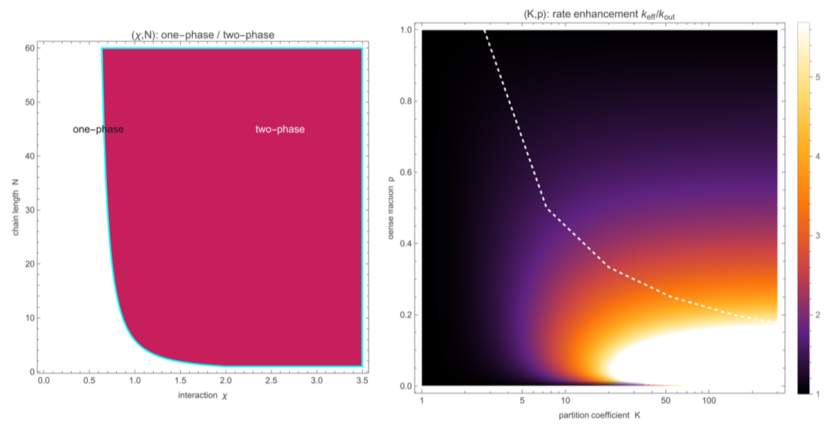
The phase behaviour of biomolecular condensates, generated live here: (left) the interaction–chain-length plane that decides whether a mixture demixes at all, and (right) how strongly a condensate accelerates the reactions inside it. Beneath it all runs a single idea — the same Flory–Huggins physics that unmixes oil from water also organises the living cell, and may have lit the first spark of life.
1. The membrane-free organelle
1. The membrane-free organelle
For over a century, cell biology was built on the assumption that the cell's internal organisation depends on membranes: lipid bilayers that enclose the nucleus, the mitochondria, the endoplasmic reticulum. Compartmentalisation by membranes was the organising principle of eukaryotic life.
Then, in 2009, Brangwynne, Eckmann, Courson, Rybarska, Hoege, Gharakhani, Jülicher, and Hyman showed that P granules — RNA–protein bodies in the germ cells of the nematode C. elegans — are not membrane-bound organelles at all. They are liquid droplets. They flow, they fuse, they drip, they dissolve and re-form. They are phase-separated condensates of RNA and proteins, held together not by a lipid membrane but by the same physics that separates oil from water.
This discovery launched a revolution. Within a decade, dozens of cellular structures were reclassified as condensates: stress granules, nucleoli, Cajal bodies, PML bodies, centrosomes, synaptic densities, heterochromatin domains, transcriptional hubs. Protein science has been transformed in parallel — the 2024 Nobel Prize in Chemistry went to David Baker for computational protein design and jointly to Demis Hassabis and John Jumper for protein-structure prediction — and the condensate revolution adds a complementary lesson: that proteins are not only rigid machines but can phase-separate into functional liquids.
The physics. The formation of a condensate is a thermodynamic phase transition. Below a critical temperature (or above a critical interaction strength), a homogeneous solution of macromolecules becomes thermodynamically unstable and spontaneously separates into a dilute phase and a dense phase. The dense phase is the condensate. The transition is governed by a competition between the entropy of mixing (which favours homogeneity) and the enthalpic interactions between molecules (which favour like-with-like aggregation). The mathematical framework for this competition is Flory–Huggins theory, which we derive in the next section.
The origin-of-life connection. Perhaps the most provocative implication of the condensate revolution is its connection to the origin of life. Aleksandr Oparin proposed (in 1924, and in molecular detail in his 1936 book) that life began inside coacervate droplets — spontaneously forming colloidal structures that concentrate organic molecules from the dilute primordial ocean. Oparin's hypothesis was dismissed for decades because the known coacervates were too disordered to sustain biochemistry. But modern condensates, with their exquisite sequence-dependent phase behaviour and their ability to concentrate specific clients by factors of up to a thousand, revive Oparin's vision in molecular detail. We show in §4 that condensate-assisted chemistry solves the concentration problem that has bedevilled prebiotic chemistry: how do you get reactions going in a picomolar ocean?
2. Thermodynamics of phase separation
2. Thermodynamics of phase separation
2.1 The Flory–Huggins free energy
2.1 The Flory–Huggins free energy
The lattice model. Consider a lattice of Nₜ sites, each occupied by either a monomer of species 1 (the polymer, chain length N₁) or a monomer of species 2 (the solvent, with N₂ = 1). Let ϕ be the volume fraction of species 1. The Flory–Huggins free energy of mixing per lattice site is:
f
kT
ϕlnϕ
N
1
(1-ϕ)ln(1-ϕ)
N
2
The first two terms are the entropy of mixing — always negative (favour mixing) and scaled by the inverse chain lengths 1/N₁ and 1/N₂. Longer chains have less translational entropy per monomer, so polymers phase-separate more readily than small molecules. The third term is the enthalpy of mixing, parameterised by the Flory interaction parameter χ. For many condensate-forming proteins, χ > 0 (unfavourable mixing) and χ decreases with temperature (χ ∝ 1/T), giving an upper critical solution temperature (UCST) phase diagram — though a substantial class of intrinsically disordered proteins (e.g. elastin-like sequences) instead show the opposite, lower critical solution temperature (LCST), behaviour.
In[]:=
figFHFreeEnergy[100,1]
Out[]=
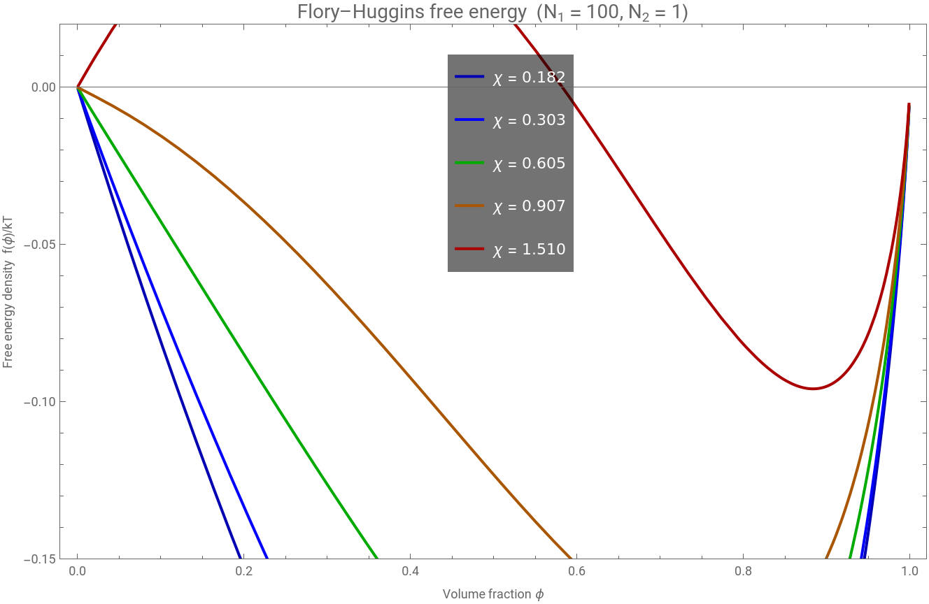
Figure 2.1 Flory–Huggins free energy density for a polymer–solvent system (N₁ = 100, N₂ = 1) at several values of χ. Below the critical χ, the free energy has a single minimum (stable mixed state). Above it, a double well appears: the system phase-separates into dilute (ϕₗ) and dense (ϕᵈ) phases at the two minima.
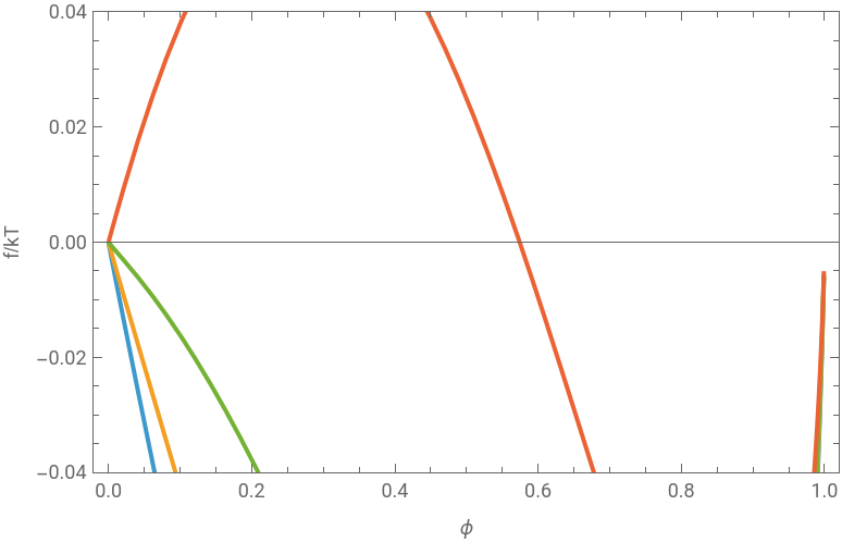
Evaluate the cell below to reproduce Figure 2.1 — the whole of Flory–Huggins is two lines of Wolfram Language:
fFH[ϕ_,n1_,n2_,χ_]:=ϕLog[ϕ]/n1+(1-ϕ)Log[1-ϕ]/n2+χϕ(1-ϕ);PlotEvaluate@Table[fFH[ϕ,100,1,χ],{χ,{0.4,0.605,0.9,1.5}}],{ϕ,0.001,0.999},
Out[]=


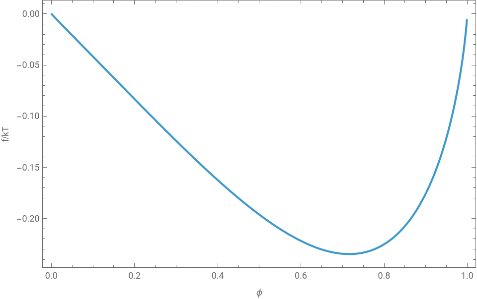
And the double well opening up as χ crosses the critical value is best felt interactively (drag χ through ≈ 0.6):
ManipulatePlotϕLog[ϕ]n1+(1-ϕ)Log[1-ϕ]+χϕ(1-ϕ),{ϕ,0.001,0.999},,{{χ,0.605,"χ"},0.3,1.6,0.005},{{n1,100,"chain length N"},1,300,1}
Out[]=


2.2 Spinodal and binodal: the phase diagram
2.2 Spinodal and binodal: the phase diagram
The thermodynamic stability of the mixed state is determined by the curvature of the free energy. The spinodal is the locus of inflection points:
2
∂
∂
2
ϕ
1
N
1
1
N
2
Inside the spinodal, the free energy has negative curvature (∂²f/∂ϕ² < 0) and the system is unstable to infinitesimal composition fluctuations — this is spinodal decomposition. Between the spinodal and the binodal (the coexistence curve), the system is metastable — it requires a finite-amplitude fluctuation (nucleation) to phase-separate.
The binodal is found by the common tangent construction: the two coexisting compositions ϕₗ and ϕᵈ satisfy equal chemical potential and equal osmotic pressure:
μ()=μ(),Π()=Π()
ϕ
L
ϕ
R
ϕ
L
ϕ
R
The critical point is where the spinodal and binodal meet:
ϕ
c
N
2
N
1
N
2
χ
c
2
1
N
1
1
N
2
2
For a long polymer (N₁ = 100, N₂ = 1): ϕᶜ = 0.091, χᶜ = 0.605. The critical concentration is low (~9%), meaning that even dilute polymer solutions phase-separate when χ exceeds a modest threshold.
In[]:=
figFHPhaseDiagram[100,1]
Out[]=
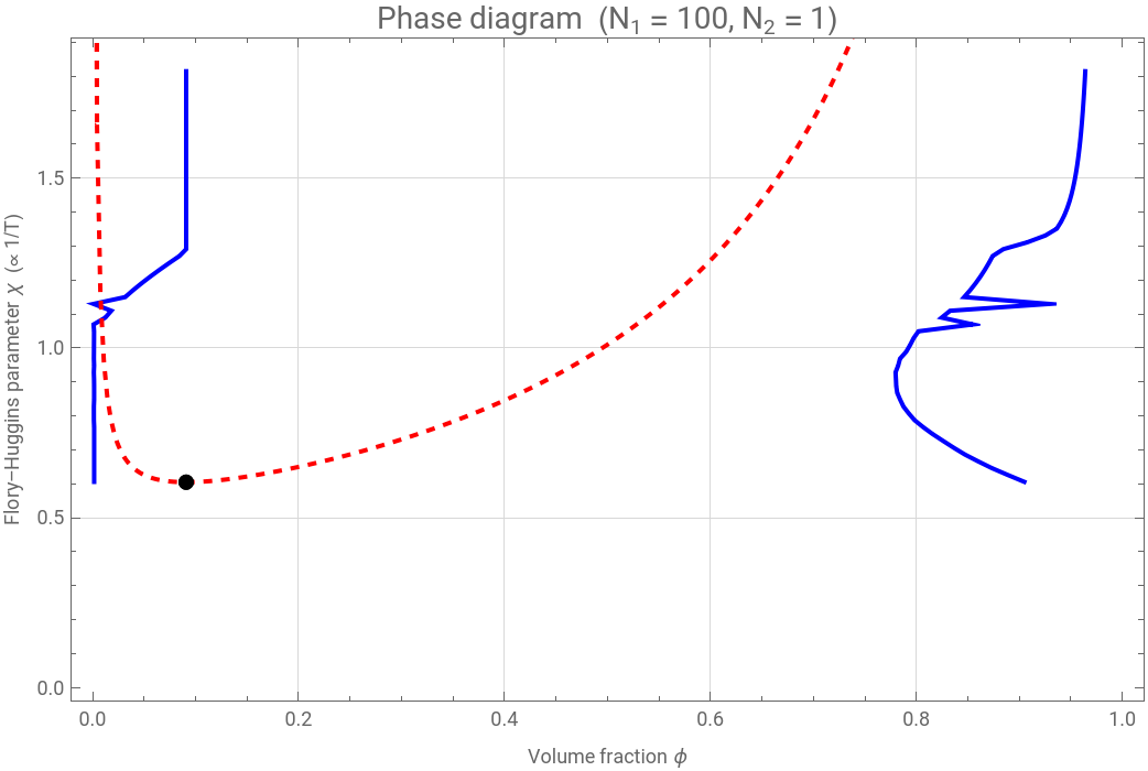


Figure 2.2 Phase diagram in χ–ϕ coordinates. The blue curve is the binodal (coexistence); the red dashed curve is the spinodal (stability limit). Between them: metastable (nucleation and growth). Inside the spinodal: unstable (spinodal decomposition). The black dot is the critical point.
2.3 Chain length and multivalency
2.3 Chain length and multivalency
A key prediction of Flory–Huggins theory is that longer polymers phase-separate more readily. The critical interaction falls toward 1/2 as chain length grows, with the excess χᶜ - 1/2 scaling as N^(-1/2): a 1000-mer demixes at χᶜ ≈ 0.53 versus ≈ 0.87 for a 10-mer, so long chains phase-separate at appreciably weaker interactions. This is biologically significant: intrinsically disordered regions (IDRs) of condensate-forming proteins are typically 50–500 residues, and their effective N is further increased by multivalent interactions (multiple binding sites per molecule, RNA scaffolds, post-translational modifications).
Figure 2.3 Spinodal curves for different chain lengths. Longer chains produce wider two-phase regions at higher temperatures (lower χ threshold). This is why proteins with long disordered regions are prone to phase separation.
3. Cahn–Hilliard dynamics of droplet formation
3. Cahn–Hilliard dynamics of droplet formation
3.1 The equation
3.1 The equation
The Flory–Huggins theory tells us whether phase separation occurs, but not how. The dynamics of a conserved order parameter (composition must be conserved — matter doesn't appear or disappear) are governed by the Cahn–Hilliard equation:
where M is the mobility (diffusion coefficient), δF/δϕ is the chemical potential from the Flory–Huggins free energy, and κ is the gradient energy coefficient that penalises sharp interfaces (it sets the surface tension γ of the condensate).
Physical content. The Cahn–Hilliard equation says: material flows down chemical potential gradients (as in ordinary diffusion), but the chemical potential now includes a penalty for composition gradients (the κ term). Inside the spinodal region, the bulk chemical potential drives uphill diffusion — material flows from dilute to concentrated regions, amplifying any fluctuation. The gradient penalty prevents infinitely sharp interfaces and selects a characteristic wavelength for the initial instability.
3.2 Spinodal decomposition
3.2 Spinodal decomposition
Figure 3.1 Top: space–time density plot of the 1D spinodal decomposition. The initially uniform composition rapidly develops concentration fluctuations that coarsen into well-separated dense (red) and dilute (blue) domains. Bottom: composition profiles at selected times showing the progression from small perturbation to fully phase-separated condensates.
3.3 Coarsening: Lifshitz–Slyozov–Wagner
3.3 Coarsening: Lifshitz–Slyozov–Wagner
Once phase separation is complete, the system continues to evolve: large droplets grow at the expense of small ones. This is Ostwald ripening, described by the Lifshitz–Slyozov–Wagner (LSW) theory. The critical radius R* is set by the Gibbs–Thomson equation:
Droplets smaller than the critical radius (R < R*) have an equilibrium concentration above the surrounding matrix supersaturation — they lose material and dissolve. Droplets with R > R* sit below it — they grow. The mean domain size grows as 〈R〉 ∝ t^(1/3), the classic LSW scaling.
Figure 3.2 Ostwald ripening of a polydisperse condensate population (100 droplets). Left: the mean and maximum droplet radius grow with time as large droplets feed on small ones. Right: the number of surviving droplets falls as the smallest dissolve — the hallmark of LSW coarsening (〈R〉 ∝ t^(1/3)).
4. Concentration enhancement and catalysis
4. Concentration enhancement and catalysis
4.1 The partition coefficient
4.1 The partition coefficient
When a condensate forms, molecules partition between the dense and dilute phases according to their chemical affinity. The partition coefficient K is defined as:
For condensate-forming proteins, K is typically 10–100. For RNA molecules that interact strongly with the condensate scaffold, K can reach 100–1000. A molecule at 1 nM bulk concentration with K = 100 is at 100 nM inside the condensate. A molecule at 1 nM with K = 1000 is at 1 μM. This is the concentration miracle.
4.2 Bimolecular rate enhancement
4.2 Bimolecular rate enhancement
For a bimolecular reaction A + B C with second-order rate constant k:
If both reactants partition equally (K_A ≈ K_B ≈ K), the reaction rate is enhanced by K². With K = 100, this is a 10⁴-fold enhancement. This is the open-system (buffered-reservoir) limit, and it is an upper bound: it assumes the surrounding dilute phase is never depleted. As §8.5 shows, imposing mass conservation caps the realised gain at order K/4. Even so, the mechanism reframes the concentration problem in prebiotic chemistry: you do not need a concentrated primordial soup if you have phase separation.
Figure 4.1 Reaction rate enhancement inside condensates as a function of the partition coefficient K, in the open-system limit (mass conservation lowers the realised gain — see §8.5). Bimolecular reactions (blue) scale as K²; the termolecular curve (red, K³) is shown only to illustrate the scaling, as three-body reactions are kinetically negligible in solution. At the typical condensate K ≈ 100, the bimolecular bound is 10⁴.
4.3 Prebiotic chemistry phase space
4.3 Prebiotic chemistry phase space
Which combinations of partition coefficient and bulk concentration allow net chemical production? We map the net replication rate (replication minus degradation) across the K–c parameter space:
Figure 4.2 Net replication rate as a function of partition coefficient K and bulk substrate concentration. The black contour marks the boundary between net growth (blue) and net decay (red). At low bulk concentrations (the likely prebiotic regime), only condensates with K > 50–100 support net replication.
5. RNA world inside condensates
5. RNA world inside condensates
5.1 Ribozyme kinetics
5.1 Ribozyme kinetics
The RNA world hypothesis proposes that the first self-replicating molecules were RNA ribozymes — RNA molecules that catalyse their own replication. The kinetics of ribozyme-catalysed replication follow Michaelis–Menten saturation:
Inside a condensate, both the enzyme (ribozyme) and the substrate (template RNA) are concentrated by the partition coefficient K. Writing Vₘₐₓ for the dilute-phase maximal rate (itself proportional to enzyme concentration), the in-condensate Vₘₐₓ is raised by the factor K (more enzyme) and the substrate concentration [S] is likewise raised by K (more substrate):
At low substrate concentrations (K [S] ≪ Kₘ), the rate scales as K² — the full bimolecular enhancement. At saturation (K [S] ≫ Kₘ), the rate scales as K (only the enzyme enhancement matters).
5.2 Replication vs degradation
5.2 Replication vs degradation
RNA is chemically unstable. In the prebiotic ocean, hydrolysis degrades RNA on timescales of hours to days. The origin-of-life window exists only when the replication rate exceeds the degradation rate:
where K* is the critical partition coefficient. Below K*, degradation wins and no self-replicating system can persist.
Figure 5.1 Replication (blue) versus degradation (red) rate as a function of the partition coefficient K, at fixed bulk substrate [S] = 1 μM. Replication is enhanced as K² and degradation as K, so above a critical K* the green-shaded origin-of-life window opens: replication outpaces hydrolysis and a self-replicating system can persist.
5.3 The origin-of-life window
5.3 The origin-of-life window
The critical partition coefficient K* depends on the ribozyme efficiency (Vₘₐₓ/Kₘ), the degradation rate constant, and the substrate level. For plausible prebiotic parameters (Vₘₐₓ ≈ 1 μM/min, Kₘ ≈ 10 μM, kᵈₑₒ ≈ 0.5/min), we find K* ≈ 10 at [S] = 1 μM, rising toward 50–100 at the lower substrate levels of a dilute prebiotic pool. Modern coacervate droplets routinely achieve K = 50–500, comfortably above this threshold — the concentration-enhancement mechanism is not marginal.
This is a quantitative version of Oparin's coacervate hypothesis: phase separation concentrates reactants enough to bootstrap biochemistry from a dilute ocean — though, as §8.5 shows, mass conservation bounds how large that boost can be.
6. Protocell dynamics
6. Protocell dynamics
6.1 Growth and division
6.1 Growth and division
A condensate droplet that sustains net internal replication grows: material produced inside increases its volume. A passive liquid droplet, however, does not divide on its own — surface tension drives it to minimise area, so it stays spherical or coalesces with its neighbours. Genuine membrane-free division requires a non-equilibrium drive: continuous chemical turnover that destabilises large droplets (Zwicker et al. 2017), or an external thermal gradient that pinches a droplet in two (§9.4; Ianeselli et al. 2022). In the toy protocell model of this section we therefore impose division as a simple size threshold — a stand-in for those mechanisms — and ask what population dynamics follow.
Figure 6.1 Schematic of the protocell life cycle. Small condensates grow by accretion of material from the bulk and by internal replication. When they exceed a critical size, an imposed threshold — standing in for the chemically- or thermally-driven fission of §9 — splits them into two daughters. Daughters inherit (with variation) the parent's composition, including its partition coefficient K and replication efficiency. Weaker daughters dissolve; fitter ones survive and grow.
6.2 Proto-Darwinian selection
6.2 Proto-Darwinian selection
If daughter droplets inherit their parent's chemical composition (approximately), and if that composition affects their fitness (replication rate, stability), then we have the three ingredients of natural selection: variation (daughters differ slightly from each other), inheritance (daughters resemble parents more than random droplets), and differential fitness (some compositions grow faster than others). This is proto-Darwinian selection — natural selection operating on condensate populations before the invention of genetic material.
We simulate this by initialising a population of 50 protocells with random partition coefficients K and replication rates, then letting them grow, divide, compete for resources, and either survive or dissolve:
Figure 6.2 Proto-Darwinian selection in a simulated protocell population. Left: mean partition coefficient K increases over time as protocells with higher K out-compete those with lower K. Centre: mean replication rate increases. Right: lineage depth (max generation number) grows as successful lineages proliferate. These trends are the signature of adaptive evolution operating on membrane-free liquid droplets.
7. Condensates and disease
7. Condensates and disease
7.1 Liquid to gel to aggregate
7.1 Liquid to gel to aggregate
Functional condensates are liquid: they flow, they exchange material rapidly with the surrounding cytoplasm, and they dissolve when the cell no longer needs them. But this liquidity is not guaranteed. Over time, or in the presence of disease-associated mutations, condensates can undergo a maturation transition: liquid gel solid aggregate. The gel state has reduced dynamics; the solid aggregate is essentially irreversible.
This maturation is implicated in several neurodegenerative diseases, though the pathologies differ. FUS and TDP-43 form functional liquid condensates whose mutated or mislocalised forms harden into the cytoplasmic inclusions of ALS and frontotemporal dementia (FTLD); tau matures into the neurofibrillary tangles of Alzheimer's and other tauopathies. (The amyloid plaques of Alzheimer's, by contrast, are built from a different peptide, amyloid-β.) In each case disease mutations or conditions shift the phase boundaries, accelerating the liquidgelsolid transition toward these pathological end states.
We model this as a three-state kinetic system:
Figure 7.1 Three kinetic scenarios for condensate ageing. Left: wild-type protein with slow maturation (healthy neuron). Centre: risk variant with moderate rates. Right: disease mutant (FUS/TDP-43 in ALS) with fast maturation — the liquid phase is rapidly depleted, and toxic aggregates accumulate.
7.2 Phase diagram of material states
7.2 Phase diagram of material states
The condensate material state depends on protein concentration and temperature (or interaction strength). We construct a schematic phase diagram showing the four regimes: mixed (one phase), liquid condensate, gel, and solid aggregate. Disease mutations effectively shift the boundaries, expanding the gel and aggregate regions at the expense of the functional liquid state.
Figure 7.2 Condensate material state phase diagram. Higher concentration and lower temperature (stronger interactions) drive the progression from mixed solution to liquid condensate to gel to solid aggregate. Disease mutations shift the boundaries toward lower concentrations and higher temperatures, making pathological aggregation more likely.
8. Nonlinear dynamics: stability, bifurcation, and coarsening
8. Nonlinear dynamics: stability, bifurcation, and coarsening
The previous sections built the model; here we analyse it with the toolkit of nonlinear dynamics — linear stability, bifurcation theory, Lyapunov functionals, and scaling laws. Every figure in this section is generated by wolfram/nonlinear_dynamics.wls (with a parallel Python implementation in src/nonlinear_analysis.py).
8.1 Linear stability and the dispersion relation
8.1 Linear stability and the dispersion relation
A uniform state is unstable precisely when f′′(ϕ₀) < 0 — the spinodal condition — in which case modes with 0 < k < k_c = sqrt(-f′′/κ) grow. The fastest-growing mode and its rate are k* = sqrt(-f′′/2κ) and ω* = M (f′′)²/4κ, setting the initial droplet spacing λ* = 2π/k*. This single mode is the seed of all condensate morphology.
The dispersion relation, live — the positive lobe (and hence the fastest-growing mode) appears exactly when f′′ < 0:
Figure 8.1 Cahn–Hilliard dispersion relation for the Flory–Huggins free energy (χ = 1.5). Curves with a positive lobe are unstable; dots mark the fastest-growing mode k*. As the mean composition ϕ₀ approaches the spinodal edge, the growth rate collapses to zero and the selected wavelength diverges.
8.2 Mode selection across the parameter plane
8.2 Mode selection across the parameter plane
The selected wavelength λ* = 2π sqrt(2κ/(-f′′)) grows with the surface-tension parameter κ and diverges at the spinodal boundary, where f′′ 0. The map below shows how the length scale is selected jointly by composition and κ.
Figure 8.2 Fastest-growing wavelength λ* over the (ϕ₀, κ) plane (clipped at 25 for contrast). The white curve is the spinodal f′′ = 0; outside it the homogeneous state is linearly stable and no length scale is selected.
8.3 Bifurcation: common-tangent coexistence vs. the spinodal
8.3 Bifurcation: common-tangent coexistence vs. the spinodal
Figure 8.3 (a) Flory–Huggins phase diagram: binodal (coexistence, blue) outside the spinodal (instability, red dashed), meeting at the critical point; the orange dot marks the solver operating point (ϕ = 0.3, χ = 1.5). (b) The symmetric double-well pitchfork, with the metastable region between binodal and spinodal.
8.4 The free energy as a Lyapunov functional
8.4 The free energy as a Lyapunov functional
8.5 Mass-conserving reaction enhancement
8.5 Mass-conserving reaction enhancement
The enhancement vanishes at both p 0 (no condensate) and p 1 (everything uniform); it is maximal at an intermediate dense fraction p* ≈ 1/K, where the gain is only ≈ K/4 — not the naive K². Bulk depletion is the hard ceiling on condensate catalysis, and it predicts an optimal droplet volume fraction — a falsifiable, quantitative claim.
Figure 8.5 Mass-conserving rate enhancement k_eff/k_out. (a) Dependence on the partition coefficients at fixed dense fraction p = 0.05. (b) Dependence on dense fraction for several K: each curve peaks at p* ≈ 1/K with a maximum gain of order K/4, far below the open-system K².
9. Active and chemically-maintained condensates
9. Active and chemically-maintained condensates
Living condensates are not at equilibrium: ATP-driven reactions continually build up and break down their components. This section extends the model with chemistry. Code: src/active_models.py, src/fh_extensions.py, and wolfram/active_dynamics.wls.
9.1 Reaction-arrested coarsening
9.1 Reaction-arrested coarsening
Add a linear chemical reaction that interconverts droplet material and a soluble form, s(ϕ) = k_+(1-ϕ) - k_-ϕ = -k_react(ϕ-ϕ_ss), to the conserved dynamics:
The reaction adds a uniform -k_react to the growth rate, ω(k) = -Mk²(f′′+κk²) - k_react, which stabilises the long-wavelength modes: the unstable band becomes finite and a length scale is selected. Ostwald ripening is arrested and the system settles into a steady-state emulsion — the mechanism behind chemically-active droplets (Zwicker et al. 2015; Bauermann et al. 2025).
Figure 9.1 Reaction-modified dispersion relation. Increasing the reaction rate pushes the small-k (long-wavelength) modes below zero, leaving a finite unstable band — coarsening can no longer proceed to arbitrarily large domains.
Figure 9.2 1D reaction–Cahn–Hilliard (NDSolve). (a) Without reaction the domains coarsen toward a single domain. (b) With reaction the pattern freezes into a steady-state periodic structure of selected wavelength.
The full 2D problem (solved with a spectral method in src/active_models.py) sharpens the same picture: chemical turnover turns the coarse, ever-growing morphology into a fine steady-state emulsion whose mean droplet size shrinks with reaction rate, and whose size distribution is narrower than the passive LSW one (Bauermann et al. 2025).
9.2 Active Model B: broken detailed balance
9.2 Active Model B: broken detailed balance
A genuinely non-equilibrium term λ|∇ϕ|² added to the chemical potential breaks detailed balance (Active Model B; Tjhung et al. 2018). Measured honestly, this term shifts the coexistence densities asymmetrically (the dense phase becomes denser than the dilute phase is dilute) and modestly slows coarsening, but does not by itself arrest it — the robust route to a steady-state emulsion is the chemical reaction of §9.1.
9.3 Stickers and spacers: multivalency drives phase separation
9.3 Stickers and spacers: multivalency drives phase separation
Real biomolecules interact through specific, saturable contacts ("stickers" joined by flexible "spacers"; Harmon & Pappu 2017). Adding a saturable association free energy f_bond = ϕ_s [ln(1-p)+p/2] (bond fraction p from the law of mass action p/(1-p)² = K_a ϕ_s, ϕ_s = vϕ) to the Flory–Huggins free energy expands the two-phase region and lowers the critical interaction: higher sticker valence v makes phase separation far easier.
Figure 9.3 Stickers-and-spacers spinodal curves. Each curve bounds the two-phase region; increasing sticker valence pushes the critical point down and outward — multivalency drives liquid–liquid phase separation even when simple mixing is unfavourable.
9.4 Thermal-gradient fission: membrane-free division
9.4 Thermal-gradient fission: membrane-free division
A temperature gradient makes the interaction χ ~ 1/T position-dependent. A warm band (weakened cohesion) drawn through an elongated droplet dissolves its neck and splits it into two daughters — division without a membrane, a candidate protocell mechanism (Ianeselli 2022). The split is genuinely band-driven: two domains form with the band, only one without it.
Figure 9.4 Thermal-gradient fission (1D Cahn–Hilliard, NDSolve). (a) At uniform temperature a single domain persists. (b) A central warm band, where the well depth a(x) dips below zero, dissolves the neck and splits the domain into two daughters — membrane-free division.
9.5 The dispersion surface
9.5 The dispersion surface
Finally, the linear-stability result of §8 viewed as a surface: the growth rate ω(k,ϕ_0) over the whole plane of wavenumber and composition, with the neutral-stability ridge ω=0 marking the boundary of the unstable region.
Figure 9.5 The Cahn–Hilliard dispersion surface ω(k, ϕ₀) for the Flory–Huggins free energy. The unstable dome shrinks to nothing as the composition approaches the spinodal edge; the cyan curve is the neutral-stability ridge.
10. Emergent complexity: selection, patterns and cycles
10. Emergent complexity: selection, patterns and cycles
The final layer of the model lets genuinely life-like behaviour emerge from the same physics. Code: src/multicomponent.py, src/darwinian_selection.py, src/reaction_diffusion_cargo.py, src/wet_dry_cycling.py, src/parameter_space.py, and the Wolfram companion wolfram/phase3_extensions.wls.
10.1 Multi-component condensates
10.1 Multi-component condensates
Real condensates contain dozens of macromolecules. For N mutually attracting components that co-condense in near-stoichiometric proportions, the demixing entropy is reduced as if they were one effective polymer of length N, and the symmetric Flory–Huggins critical point migrates (Qian & Knowles 2022):
As N grows the critical concentration falls toward zero — multivalent mixtures phase-separate at vanishing concentration — and the critical interaction drops, so they demix far more easily. Distinct scaffolds give distinct condensates, and each client partitions selectively into the one it binds best (the physical basis of organelle identity).
Figure 10.2 Selective compartmentalisation: a ternary (A, B, solvent) free energy in which two mutually-repelling solutes form an A-rich and a B-rich condensate — each client partitions into the droplet it binds best, the physical basis of organelle identity.
10.2 Darwinian selection among protocells
10.2 Darwinian selection among protocells
The intellectual climax. Replicators partition into condensate droplets and replicate at a rate set by a heritable genotype g, competing for a shared global nutrient under a uniform chemostat dilution. Replicators whose growth rate r_0 g falls below the dilution rate are out-competed (competitive exclusion), and the population's mean fitness climbs. A full 2D spatial version (src/darwinian_selection.py), in which fuel-driven droplets grow, divide under periodic thermal pulses, and pass their genotype to daughters, reaches the same outcome with explicit lineages.
The result is natural selection from pure physics. The cargo-weighted mean fitness rises over generations and saturates at a mutation-selection balance — no biology is hand-coded; selection is an emergent consequence of the dynamics.
What the selection requires. The effect is not automatic: it demands Malthusian (per-capita) replication competing for a shared, global nutrient together with a uniform chemostat dilution. Replacing the shared resource with a local carrying capacity, or raising the mutation rate too high, erases the inheritance signal — mean fitness then drifts rather than climbs and selection collapses. The trajectory below is therefore a genuine result of the chosen ecology, not a foregone conclusion.
Figure 10.3 Chemostat competition (NDSolve). Left: the population's mean fitness 〈g〉 rises toward g_max as fitter replicators take over. Right: the fittest genotype out-competes the rest — competitive exclusion, with no biology hand-coded.
Figure 10.4 A protocell phylogeny generated by the same selection dynamics: fit (yellow) lineages branch and proliferate while low-fitness (blue) lineages die out (node colour = fitness).
10.3 Reaction-diffusion inside condensates
10.3 Reaction-diffusion inside condensates
A condensate is also a chemical reactor. When crowding slows the activator far more than the inhibitor, the diffusion ratio D_v/D_u crosses the Turing threshold only inside the dense phase: a band of wavenumbers becomes unstable there while every mode stays stable in the dilute surroundings, so spots self-organise inside the condensate and nowhere else. (The full 2D patterns, and the reaction hotspot that forms in a shell at the droplet interface, are computed in src/reaction_diffusion_cargo.py.)
Figure 10.5 Schnakenberg linear-stability growth rate λ(k): inside the dense phase a band of wavenumbers is unstable (patterns form), while in the dilute phase every mode is stable. The Turing instability is switched on by the condensate.
10.4 Wet-dry cycling
10.4 Wet-dry cycling
On the early Earth, rock pools cycled between flooded (wet) and evaporated (dry) states. Cycling the interaction χ(t)=χ_0+Δχ sin(2πt/T) swings the system between a one-phase well (dissolve, remix) and a spinodally unstable double well (re-nucleate many droplets). Each dissolution erases the size differences that drive Ostwald ripening, so a population of droplets is maintained, while a matched constant-χ run coarsens toward a single winner (Ianeselli 2022).
Figure 10.6 1D wet–dry Cahn–Hilliard space–time (NDSolve): with a cyclic well depth a(t), domains dissolve at each wet half-cycle and re-nucleate at each dry half-cycle. The repeated dissolution resets the size differences that would otherwise drive Ostwald ripening, so a population of droplets is sustained rather than coarsening to a single winner (Ianeselli et al. 2022).
10.5 The accessible parameter space
10.5 The accessible parameter space
Finally, two analytic maps of the model's regimes: the (χ,N) plane separating one-phase from two-phase by the critical line χ_c(N), and the (K,p) mass-conserving rate-enhancement landscape with its optimal ridge p*≈1/K. (The full four-panel regime atlas — which also includes the thermodynamic (ϕ_0,κ) plane and the active dissolution / microphase / macrophase plane from 2D simulations — is built in src/parameter_space.py.)
Figure 10.7 The two analytic regime planes. Left, (χ,N): the one-phase / two-phase boundary along the critical line. Right, (K,p): the mass-conserving rate enhancement, with the optimal ridge p*≈1/K (dashed).
11. Conclusions
11. Conclusions
The bigger picture. Biomolecular condensates sit at the intersection of soft-matter physics, molecular biology, the origin of life, and neurodegeneration. The mathematical framework — Flory–Huggins thermodynamics, Cahn–Hilliard dynamics, Michaelis–Menten kinetics, Lifshitz–Slyozov coarsening — is classical and well-understood. What is new is the recognition that this physics operates inside living cells, that it provides the thermodynamic foundation for protocellular compartments, and that its failure modes are disease. The condensate revolution is not a discovery of new physics; it is the discovery that old physics was hiding in plain sight inside biology.
Key takeaways.
◼
Phase separation is thermodynamics, not biology. A two-parameter Flory–Huggins free energy already predicts when proteins and RNA demix into condensates.
◼
Concentration is the payoff — but it is bounded. Partitioning boosts bimolecular rates by up to K² in the open-system limit, while mass conservation caps the realised gain at order K/4.
◼
Life-like behaviour is emergent. Add chemistry, heredity and a shared resource and natural selection, Turing patterns and ripening-resistant populations fall out of the same equations — no biology hand-coded.
◼
The same physics, run backwards, is disease. The liquidgelsolid maturation that endangers neurons is the flip side of the transition that organises healthy cells.
12. References
12. References
Qian, D., Michaels, T. C. T., & Knowles, T. P. J. (2022). Analytical solution to the Flory–Huggins model for multicomponent phase separation. Journal of Physical Chemistry Letters 13, 7853–7860. [Multi-component critical point.]
Turing, A. M. (1952). The chemical basis of morphogenesis. Philosophical Transactions of the Royal Society B 237, 37–72. [Reaction-diffusion patterns.]
Eigen, M. (1971). Selforganization of matter and the evolution of biological macromolecules. Naturwissenschaften 58, 465–523. [Competitive exclusion of replicators.]
Ianeselli, A., Atienza, M., Kudella, P. W., et al. (2022). Water cycles dissolve and divide protocell-like droplets. Nature Chemistry 14, 32–39. [Wet-dry cycling and thermal fission.]
Flory, P. J. (1942). Thermodynamics of high polymer solutions. Journal of Chemical Physics 10, 51–61.
Huggins, M. L. (1942). Some properties of solutions of long-chain compounds. Journal of Physical Chemistry 46, 151–158.
Cahn, J. W., & Hilliard, J. E. (1958). Free energy of a nonuniform system. I. Interfacial free energy. Journal of Chemical Physics 28, 258–267.
Lifshitz, I. M., & Slyozov, V. V. (1961). The kinetics of precipitation from supersaturated solid solutions. Journal of Physics and Chemistry of Solids 19, 35–50.
Oparin, A. I. (1924). Proiskhozhdenie Zhizni (The Origin of Life). Moscow: Moskovskii Rabochii.
Brangwynne, C. P., Eckmann, C. R., Courson, D. S., Rybarska, A., Hoege, C., Gharakhani, J., Jülicher, F., & Hyman, A. A. (2009). Germline P granules are liquid droplets that localize by controlled dissolution/condensation. Science 324, 1729–1732. [The founding observation.]
Hyman, A. A., Weber, C. A., & Jülicher, F. (2014). Liquid–liquid phase separation in biology. Annual Review of Cell and Developmental Biology 30, 39–58.
Banani, S. F., Lee, H. O., Hyman, A. A., & Rosen, M. K. (2017). Biomolecular condensates: organisers of cellular biochemistry. Nature Reviews Molecular Cell Biology 18, 285–298. [Comprehensive review.]
Shin, Y., & Brangwynne, C. P. (2017). Liquid phase condensation in cell physiology and disease. Science 357, eaaf4382.
Patel, A., Lee, H. O., Jawerth, L., et al. (2015). A liquid-to-solid phase transition of the ALS protein FUS accelerated by disease mutation. Cell 162, 1066–1077. [Disease connection.]
Zwicker, D., Seyboldt, R., Weber, C. A., Hyman, A. A., & Jülicher, F. (2017). Growth and division of active droplets provides a model for protocells. Nature Physics 13, 408–413. [Protocell dynamics.]
Dignon, G. L., Zheng, W., Best, R. B., Kim, Y. C., & Mittal, J. (2018). Relation between single-molecule properties and phase behavior of intrinsically disordered proteins. Proceedings of the National Academy of Sciences 115, 9929–9934.
Wagner, C. (1961). Theorie der Alterung von Niederschlägen durch Umlösen (Ostwald-Reifung). Zeitschrift für Elektrochemie 65, 581–591. [The "W" in LSW coarsening.]
Zwicker, D., Hyman, A. A., & Jülicher, F. (2015). Suppression of Ostwald ripening in active emulsions. Physical Review E 92, 012317. [Chemically active droplets.]
Tjhung, E., Nardini, C., & Cates, M. E. (2018). Cluster phases and bubbly phase separation in active fluids: reversal of the Ostwald process. Physical Review X 8, 031080. [Active Model B.]
Harmon, T. S., Holehouse, A. S., Rosen, M. K., & Pappu, R. V. (2017). Intrinsically disordered linkers determine the interplay between phase separation and gelation in multivalent proteins. eLife 6, e30294. [Stickers and spacers.]
Schnakenberg, J. (1979). Simple chemical reaction systems with limit cycle behaviour. Journal of Theoretical Biology 81, 389–400. [Reaction–diffusion model.]
Bauermann, J., Bartolucci, G., Weber, C. A., & Jülicher, F. (2025). The droplet size distribution and its dynamics in chemically active emulsions. Physical Review Letters 135, 148201. [Active-emulsion size distributions.]
Further reading
Further reading
For an accessible, non-technical tour of the same story – condensates, coacervates and the idea that the origin of life may have been hiding inside our own cells all along – see the New Scientist cover feature that prompted this notebook:
Marshall, M. (2026). Hiding in plain sight. New Scientist, 20 June 2026, pp. 30–33 (Features / Cover story). Online edition titled “Has the answer to life’s origins been hiding in our cells all along?” newscientist.com/article/2529162 (https://www.newscientist.com/article/2529162-has-the-answer-to-lifes-origins-been-hiding-in-our-cells-all-along/).
13. Reproducibility
13. Reproducibility
All source code lives in the repository https://github.com/mthiel74/biomolecular-condensates. The pipeline has two parallel tracks: Wolfram Language (analysis scripts in wolfram/ and this notebook builder in community/) and Python (src/, including a full 2D Cahn–Hilliard spectral solver). The figures come from both tracks: the Wolfram scripts write directly to docs/images/, while the Python scripts write to figures/ and are copied across. Wolfram Language 13+ is required. To regenerate this notebook from scratch, run the Python track first, then the Wolfram runner (which now also executes the Phase-3 companion and copies the Python figures into place), then the builder:
# 1. Python track ⟶ writes figures to figures/
pip install -r src/requirements.txt # numpy, scipy, matplotlib (+ ffmpeg for animations)
python3 src/flory_huggins.py
python3 src/cahn_hilliard.py
python3 src/condensate_kinetics.py
python3 src/protocell.py
python3 src/nonlinear_analysis.py # nonlinear-dynamics analysis (§8)
python3 src/fh_extensions.py # stickers-and-spacers (§9.3)
python3 src/active_models.py # active condensates (§9)
python3 src/multicomponent.py # multi-component condensates (§10.1)
python3 src/darwinian_selection.py # Darwinian selection (§10.2)
python3 src/reaction_diffusion_cargo.py # reaction-diffusion (§10.3)
python3 src/wet_dry_cycling.py # wet-dry cycling (§10.4)
python3 src/parameter_space.py # parameter space (§10.5)
python3 src/phase3_heroes.py # hero visualisations
# 2. Wolfram analysis + copy of Python figures ⟶ docs/images/
wolframscript -file wolfram/run_all.wls
# 3. Rebuild this notebook
wolframscript -file community/build_notebook.wls
Licence and provenance. All code and every figure in this notebook are original and generated by the accompanying scripts; the notebook and figures are released under the MIT licence (see LICENSE in the repository). Suggested Wolfram Community tags: Biology, Physics, Differential Equations, NDSolve, Phase Transitions, Origin of Life, Soft Matter.
Generated on June 26, 2026 with Wolfram Language 15..
CITE THIS NOTEBOOK
CITE THIS NOTEBOOK
Biomolecular condensates: Flory-Huggins thermodynamics and liquid-liquid phase separation origins
by Marco Thiel
Wolfram Community, STAFF PICKS, June 26, 2026
https://community.wolfram.com/groups/-/m/t/3739768
by Marco Thiel
Wolfram Community, STAFF PICKS, June 26, 2026
https://community.wolfram.com/groups/-/m/t/3739768