ABSTRACT (original article): In rigid origami, the complex folding motion arises from the rotation of strictly rigid faces around crease lines that represent perfect revolute joints. The rigid folding motion of an origami crease pattern is collectively determined by the kinematics of its individual vertices. Establishing a kinematic model and determining the conditions for the rigid foldability of a single vertex is thus important to exploit rigid origami in engineering design tasks. Today, there exists neither an efficient kinematic model to determine the unknown dihedral angles nor an intrinsic condition for the rigid foldability of arbitrarily complex vertices of degree n. In this paper, we present the principle of three units (PTU) that provides an efficient approach to modeling the kinematics of single degree-n vertices. The PTU is based on the notion that the kinematics of a vertex is determined by the behavior of a single underlying spherical triangle. The condition for the existence of this triangle leads to the condition for the rigid and flat foldability of degree-n vertices. These findings are transferred from single vertices to crease patterns, resulting in a simple rule to generate kinematically determinate crease patterns that can be designed to fold rigidly. Finally, we discuss the limitations of the PTU with respect to the global rigid foldability of a crease pattern. CITATION (original article): Zimmermann, L., Shea, K., and Stanković, T. (October 31, 2019). “Conditions for Rigid and Flat Foldability of Degree-n Vertices in Origami.” ASME. J. Mechanisms Robotics. February 2020; 12(1): 011020. https://doi.org/10.1115/1.4045249
We decided to opensource this origami script for 3 reasons: first, it is useful. Second, while it returns great results, it can be optimized in certain parts and revolutionized in others (there’s unsolved geometry, help!). Third, the corresponding paper [1], while readable, was written in research fashion: devoid of fun and philosophy. So, let us try again.
We find ourselves in the world of rigid origami, where rigid bodies connected by rigid joints underlying rigid mathematics are still able to perform motion - just like a door. A door (Fig. 1, left), commonly a hard piece of wood turning on stiff metal hinges fixed to a stationary axis, turns for half a rotation into one, sometimes even two directions, and comes to rest only when it hits a wall; a motion that is both highly efficient and slightly boring. Note, the boringness stems not from the presence of a predictable motion but from the absence of a rich one, which can be achieved by introducing one tiny rule: each and every rotational axis, or fold line, cannot span the entirety of the paper (Fig. 1, middle) but must meet other folds before leaving the paper (Fig. 1, right). Then, we call it a rigid origami.
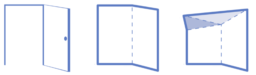
Fig. 1
“Meeting other folds” might lead to the impression that multiple folds just randomly meet at the same exact point, which would be a wild coincidence, and thus not entirely intuitive. Better think of a fold entering the paper like a break in the ice. First, it travels in a straight line (Fig. 2a), but at some point and for whatever reason it cannot continue straight, and so it splits into new folds (Fig. 2b). Each new fold travels in a straight line and may either reach a crossing-point where it splits again (Fig. 2c) or encounter other folds to make baby folds (Fig. 2d), until at last it dies at the end of the paper (Fig. 2e). That’s the life of a fold: alternating between lonesome travels and intervals of sudden reproductions. And like in real life, these reproductions are madly interesting, so interesting that we can forget the lonely times of travel, or in other words, the entire information of an origami is encoded within its vertices, and our goal here is to decode this information to understand the principle of folding on a deep, intuitive level.
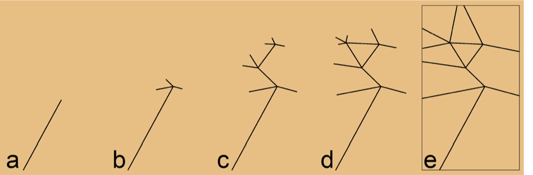
Fig. 2
Let us introduce the mathematical foundation for the simplest of vertices, a degree-4 vertex (Fig. 3), and then generalize for all vertices. The degree of a vertex is defined by the number of meeting fold lines or crease lines. The behavior of a vertex is defined by the angles between its crease lines, called the sector angles α, which, once defined by us, are fixed throughout the entire folding motion to preserve the rigidity of the origami. In comparison to the fixed sector angles, the dihedral angles ρ, which describe the rotation around the crease lines, change over time and thus represent the current state of motion. To achieve this motion, however, we need to first drive the folding process by controlling at least one dihedral angle ρ, and in the case of a degree-4 vertex, it is exactly one driving angle (ρ1 in Fig. 3) that controls the three yet unknown dihedral angles (ρ2, ρ3, and ρ4).
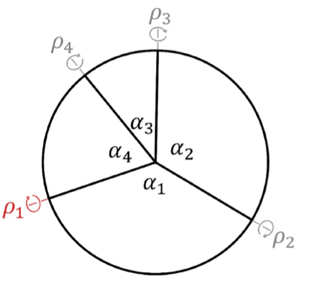
Fig. 3 [2]
How do we know that degree-4 vertices require a single driving angle? It is a long-standing fact that any degree-n vertex requires n-3 driving angles to uniquely determine its motion. We must confess here that, historically, we have focused on the wrong part of this equation, the n-part, until we finally realized that the 3 is more important, because it means that independent of the number of driving angles, independent of the degree, and thus generally true for any degree-n vertex, there must always be 3 unknowns. We can present the same statement in a slightly different light, as colorfully depicted in Fig. 4. In the top left corner we show an arbitrary degree-4 vertex, n = 4. The single driving angle is symbolized by an arrow that shows at which crease line the driving force acts, i.e. where the folding takes place. Now suppose we fold the highlighted crease line, i.e. we hold the left blue sector with our left hand and the right blue sector with our right hand and bend around the arrowed crease line, then, while it is hard to predict the motion of the yellow and red sectors, we know exactly what the blue sectors will do, since we fold them, right? In mathematical terms, the behavior of the blue section is fully determined by our input and thus gets one and the same color. In general, the simple rule to assign colors thus says that the sectors adjacent to a driving angle get the same color. In the top right corner of Fig. 4, one more crease line is added in order to create a degree-5 vertex, which requires 2 driving angles, again symbolized by arrows. Depicted from left to right in n = 5 are possible combinations of arrow locations, and since we are only interested in the relative location of one arrow to the other, these states depict all existing combinations (e.g., the current distribution ((1, 2), (1, 3), (1, 4), (1, 5)) is identical to ((2, 3), (2, 4), (2, 5), (2, 1)) or any other permutation). For the left-most vertex in n = 5, the motion of the red and yellow sectors are again hard to predict while the state of the entire blue chain of sectors is determined by our input of driving angles. When proceeding to the next vertex in line, for the first time we control two chains of sectors, the blue and the red one, then we control the blue and yellow one, before we return to only one blue chain being controlled. The same color distribution shows for the degree-6 vertex and all subsequent vertices: independent of the distribution of n-3 driving angles, a rigidly foldable vertex is always comprised of 3 colors, chains of sectors, or units. This is the essence of the Principle of Three Units (PTU).
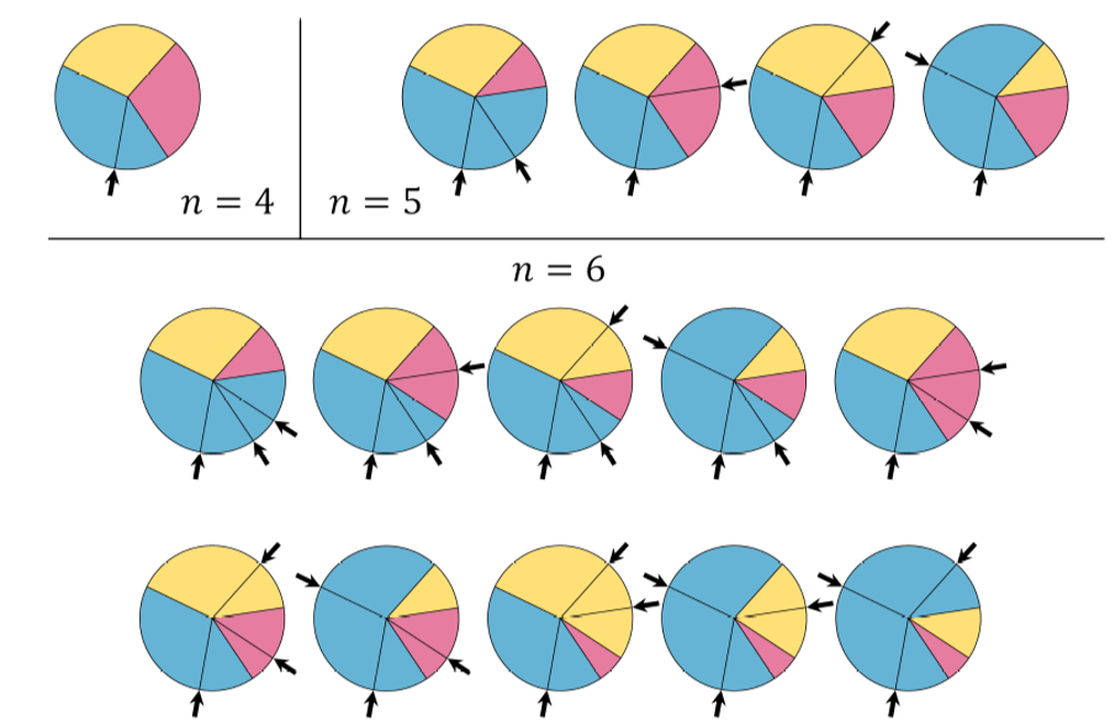
Fig.4
The simplicity of this realization is anti-proportional to its impact: instead of seeing a vertex as a complicated assemblage of three-dimensional rotations, we can perceive the three units as the three sides of a simple, spherical triangle. In consequence, all important equations are well-known and long-established, and many unintuitive facts suddenly make sense (more to that later). Let us visually internalize the PTU by an example illustrated in Fig. 5 where we dissect a vertex into its parts. Fig. 5a shows an arbitrary degree-8 vertex with 5 driving angles highlighted as black arrows. (Again, driving a different set of crease lines is possible as long as there are 5.) In-between these driving angles lie the 3 unknown dihedral angles in grey, whose determination is our long-term goal to determine the kinematic equations, but for now we cut them free, just like in basic mechanics. Doing so results in Fig. 5b, where the three units u1, u2, and u3 emerge together with their most important characteristic, the unit angle U, which spans the entire unit from its first to its last crease line. In this example, two of three unit angles are driven, i.e. time-dependent, (0) and (0) shown at t=0, while is constant and equal to the size of the sector angle . As soon as the folding motion is introduced, the unit angles deviate from their initial state (Fig. 5c) and, since the surface around the vertex must be continuous, form a spherical triangle (Fig. 5d), which we call the vertex triangle.
U
1
U
2
U
3
α
8
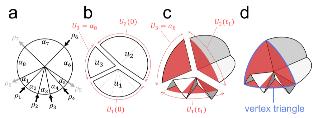
Fig. 5 [1]
For each and every vertex there exist two of these vertex triangles. Why? Because a triangle with three given, ordered sides has two possible shapes. Figure 6 left shows the planar case, where two of the sides can coincide in the points C1 and C2. The right-hand side of Fig. 6 shows the equivalent case for an origami vertex, where two vertex triangles are possible, one “up” and one “down” (note, all driving angles are identical in “up” and “down”). Thus, instead of seeing an origami vertex as a complicated assemblage of mountain-valley assignments, we can perceive it as a binary state of two triangles, rigid body modes, or just modes.
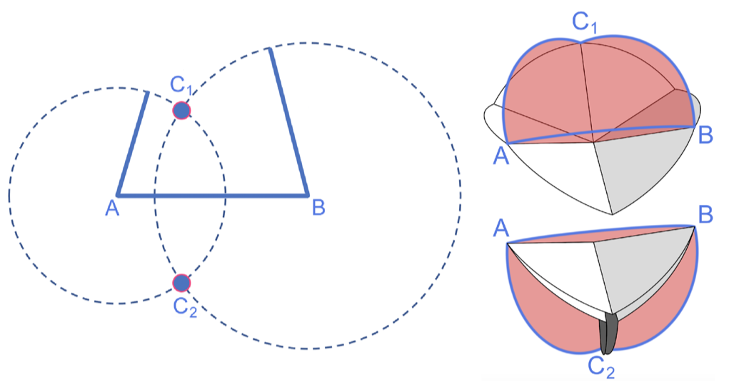
Fig. 6 [adapted from 1]
Let us now start to embed the story in code. Our goal will be to model the kinematics of an origami vertex by the following (exemplary) input:
In[]:=
u1={{80Pi/180,120Pi/180},{t}};u2={{100Pi/180}};u3={{60Pi/180}};mode=0;(*or1*)
In unit u1, two sector angles of 80° and 120° are adjacent to a driving angle t representing the “time“, which is linear in this case but can adopt any kind of function. Units u2 and u3 are constant, but in general each unit can contain arbitrarily many sector and driving angles as long as there is one less driving angle than sector angles. Also, the only assumption we made so far is that the surface around the vertex is rigid, not flat, so the PTU applies to non-developable vertices, spherical R-mechanisms, as well as discrete parabolic and hyperbolic surfaces. Finally, mode adopts values 0 or 1 representing the states “up” and “down”, though these terms can be misleading depending on the shape of the vertex, because vertices can really fold in any direction - in their rigid world, they are free beings.
The output will be the three unknown dihedral angles that lie between the three units at the corners of the vertex triangle (see, e.g., Fig. 5). We start by defining the function pointCoordinates that takes two lists of sector and dihedral angles and returns all point coordinates spanned by that chain of sectors. In pointCoordinates, the rotationMatrices are first brought into alternating order, where all sectorAngles represent a rotation around the z-axis and the dihedralAngles rotate around the x-axis. Then, the rotationMatrices are dot multiplied with the startPoint to express the point coordinates. Note, the startPoint is arbitrarily chosen on the x-axis for the origin that will be placed at {0, 0, 0}.
In[]:=
pointCoordinates[sectorAngles_,dihedralAngles_]:=Module[{rotationMatrices,startPoint,pCoord},rotationMatrices=Riffle[RotationMatrix[#,{0,0,1}]&/@sectorAngles,RotationMatrix[#,{1,0,0}]&/@dihedralAngles];startPoint={1,0,0};pCoord=Table[(Dot@@rotationMatrices[[1;;i]]).startPoint,{i,1,Length[rotationMatrices],2}];PrependTo[pCoord,startPoint]]
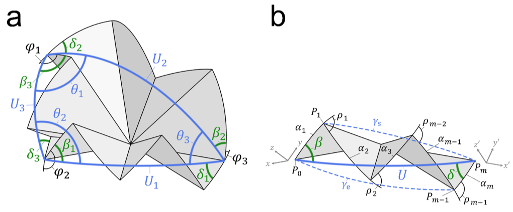
Next, we must find the puzzle piece angles that constitute the unknown dihedral angles. As illustrated in Fig. 7a, the unknowns φ (in black) lie at the corners of the vertex triangle (in blue) and are the sum of three angles: the internal angles of the vertex triangle θ (also in blue), the angles β at the start of each unit, as well as the angles δ at the end of each unit (both in green). Since the internal angles θ can just be expressed by subjecting the unit angles U to the spherical law of cosines, we are presently interested in finding U, β, and δ.
The heavy lifting is done, what remains is the culmination of our hard work. The input to the function dihedralAngles is the original input of mode and three units. By employing unitRelatedAngles, we find allAngles with which we define the betas, Us, and deltas. Then, the thetas are expressed by applying the spherical law of cosine to the vertex triangle, after which the unknownDihedralAngles can be determined by summing said angles and by rotating the thetas in both directions depending on the mode. As a last step, we bring allDihedralAngles in the correct order and delete the “noDihedralAngle”. Voilà, vertex is served.
Plotting the vertex in plotOrigami does not require explanation, worthy of note is only that our first function pointCoordinates can be re-used here to find the pointsToPlot, thereby closing the circle of code, how beautiful. Also, best don’t go to 0 or π with t, it can mess up the system. Other than that, enjoy playing around with different vertex configurations, it’s a lot of fun. To not miss out on more fun, however, read on below to get some more possibilities of the PTU.
The higher the vertex degree, the better we perceive the vertex triangle without actually plotting it, as shown in Fig. 8. Especially the last row (n = 360) exemplifies the beauty of folding, because a 2D plane folds into a 3D shape and back into a 1D line, thus reducing the dimension of the object (!). It reminds us of some crazy dimensionality reduction of matter on the horizon of a black hole, or similar, but do not cite us on this, it is just idea generation for the smarter minds out there. Can someone tag?
Here is the vertex for Fig. 8:
We can do “curved” folding:
Code for Fig. 9:
We can write stuff. Basically, we have full control over single vertices. (We did not find the code to this one, write your own stuff! Questions?)
Also, we can fold discrete hyperbolic (or parabolic) surfaces where the surface area around the vertex is greater (smaller) than 2π, see Fig. 11. Such vertices are equal to spherical R-mechanisms and thus potentially interesting for robotic applications. Note that when no triangle can be formed, Mathematica will give out a red background (Fig. 11, left), but do not get discouraged and just fold on, because as soon as the vertex triangle can be formed, the entire vertex shows (with the below code, that moment lies at ca. t = 0.85).
Code for Fig. 11:
The exemplary vertex is thus only rigidly foldable until ca. t ≈ 1.45.
Fig. 12
This equation for flat foldability allows us, e.g., to design flat foldable vertices of any degree, but especially of odd-degree, which was difficult to achieve before the insights gained from the PTU:
Code for Fig. 13:
Apropos flat, the attention span of the readers is probably also getting flat at this point, which is why we want to close with a last question: Why are we doing all this? 1. Because it is fun. 2. Because folding is a universal principle in nature and too few people are talking about it. Even if this script is restricted to rigid folding, there emerge many similarities to curved / compliant folding. 3. Because we can extend the PTU to multiple vertices and, together with the condition for rigid foldability, can design some really cool things.
Think back of the break in the ice in Fig. 2 and notice how every vertex generates 3 outgoing crease lines when splitting. As long as we satisfy the rule that every vertex has 3 outgoing crease lines and that there are no cycles in our origami crease pattern (because the PTU cannot handle cycles, which are a really interesting and un-researched topic), the design possibilities are endless. For example, we can fold 1 DOF chairs:
Or we can optimize medical grippers, as presented by the GIF at the top of this blog.
But more on how to go from single to multiple vertices in the next round, if anyone is interested. Until then, stay healthy and please close the door when leaving.
[1] Zimmermann, L., Shea, K., and Stankovic, T., "Conditions for Rigid and Flat Foldability of Degree-n Vertices in Origami", Journal of Mechanisms and Robotics 12 (1), 011020.
[2] Zimmermann, L., Stankovic, T., “Rigid and flat foldability of a degree-four vertex in origami”, Journal of Mechanisms and Robotics 12 (1), 011004.
The script can be downloaded under MIT license here: https://app.data-archive.ethz.ch/delivery/DeliveryManagerServlet?dps_pid=IE23254599
The script can be downloaded under MIT license here: https://app.data-archive.ethz.ch/delivery/DeliveryManagerServlet?dps_pid=IE23254599
CITE THIS NOTEBOOK
CITE THIS NOTEBOOK
The Principle of Three Units: intuitive approach to folding rigid origami
by Luca Zimmermann and Tino Stankovic
Wolfram Community, STAFF PICKS, March 17, 2022
https://community.wolfram.com/groups/-/m/t/2492007
by Luca Zimmermann and Tino Stankovic
Wolfram Community, STAFF PICKS, March 17, 2022
https://community.wolfram.com/groups/-/m/t/2492007