ABSTRACT (original article): Numerical models of photodissociation regions (PDRs) are an essential tool to quantitatively understand observations of massive star forming regions through simulations. Few mature PDR models are available and the Cologne KOSMA-τ PDR model is the only sophisticated model that uses a spherical cloud geometry, thereby allowing us to simulate clumpy PDRs. We present the current status of the code as a reference for modelers and for observers that plan to apply KOSMA-τ to interpret their data. For the numerical solution of the chemical problem, we present a superior Newton-Raphson stepping algorithm and discuss strategies to numerically stabilize the problem and speed up the iterations. The chemistry in KOSMA-τ is upgraded to include the full surface chemistry in an up-to-date formulation and we discuss a novel computation of branching ratios in chemical desorption reactions. The high dust temperature in PDRs leads to a selective freeze-out of oxygen-bearing ice species due to their higher condensation temperatures and we study changes in the ice mantle structures depending on the PDR parameters, in particular the impinging ultraviolet field. Selective freeze-out can produce enhanced C abundances and higher gas temperatures, resulting in a fine-structure line emission of atomic carbon [C I] enhanced by up to 50% if surface reactions are considered. We show how recent Atacama Large Millimeter Array (ALMA) observations of emission in the Orion Bar with high spatial resolution on the scale of individual clumps can be interpreted in the context of nonstationary, clumpy PDR ensembles. Additionally, we introduce WL-PDR, a simple plane-parallel PDR model written in Mathematica to act as a numerical testing environment of PDR modeling aspects. CITATION (original article): M. Röllig and V. Ossenkopf-Okada, The KOSMA-τ PDR model - I. Recent updates to the numerical model of photo-dissociated regions, A&A, 664 (2022) A67. https://doi.org/10.1051/0004-6361/202141854
+
HCO
Numerical models of photodissociation regions (PDRs) are an essential tool to quantitatively understand observations of massive star forming regions through simulations. We introduce WL-PDR, a simple plane-parallel PDR model written in Wolfram Language to act as a numerical testing environment of PDR modeling aspects.
Introduction
Introduction
Photodissociation regions (PDRs) are region sin the interstellar medium, i.e. clouds of gas and dust, where the physical and chemical conditions are dominated by the local intensity of the far UV (FUV) radiation, coming from nearby massive stars.
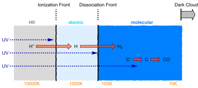
Fig . 1 Simplified structure of a PDR. UV radiation (coming from the left) is progressively attenuated while penetrating a gas cloud. This leads to a chemical stratification and a strong temperature gradient.
Numerical models of PDRs are a valuable tool to model their chemical and thermodynamic structure and to simulate their line and continuum emission in order to compare these predictions with observation to derive local conditions in the ISM. Typically, PDR models are very complex numerical models written in FORTRAN or C. Here, we introduce WL-PDR, a simple plane-parallel PDR model written in Mathematica to act as a numerical testing environment of PDR modeling aspects.
It is useful to reduce the numerical complexity of a model in order to better study numerical or physical aspects of the model. For some numerical tests in the paper Röllig & Ossenkopf-Okada (2022) we use the simple 1-D, semi-infinite plane-parallel PDR model code WL-PDR. The code is ported to Mathematica from PyPDR (Bruderer 2019). PyPDR is used as an educational tool to learn about the basic physics and some numerical internals of PDR codes. We ported PyPDR to Mathematica to seamlessly integrate the toy PDR model into our research infrastructure and to make use of the advanced analysis, numerics and visualization capabilities of Mathematica.
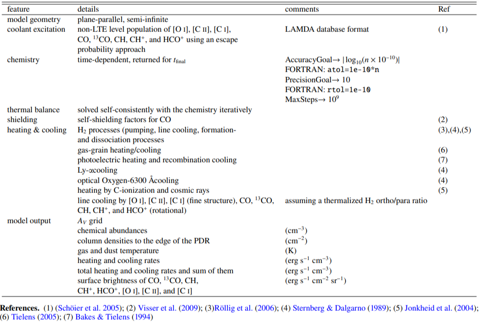
The features of WL-PDR are summarized in the following Table (Table G.1 from Röllig & Ossenkopf-Okada 2022).
The code can be downloaded at https://github.com/markusroellig/WL-PDR
Code
Code
Definitions
Definitions
Misc. definitions
Misc. definitions
Chemistry
Chemistry
Import chemical network
In[]:=
$dataDir=NotebookDirectory[];
In[]:=
raw=Import[FileNameJoin[{$dataDir,"data_chemnet.dat"}],"Table"];(*numberofelements*)nelem=raw[[2]]//Flatten//First(*numberofchemicalspecies*)nspecies=raw[[4+nelem+1]]//Flatten//First(*numberofchemicalreactions*)nreactions=raw[[7+nelem+nspecies+1]]//Flatten//First
Out[]=
6
Out[]=
31
Out[]=
307
CO self shielding factors (shielding from FUV radiation).
In[]:=
rawSS=Import[FileNameJoin[{$dataDir,"data_coselfs.dat"}],"Table"];COselfs:=ListInterpolationrawSS,logspace[,,42],logspace[,,47]COselfs[,]
14.8
10
23.
10
9.8
10
19.
10
23
10
19
10
Out[]=
3.306×
-7
10
Species, their relative elemental abundance (relative to H) and their elemental composition.
In[]:=
species=raw[[6+nelem+1;;6+nelem+nspecies]]
Out[]=
{{H,1.,1,0,1,0,0,0},{H+,0.,1,1,1,0,0,0},{H2,0.,2,0,2,0,0,0},{H2+,0.,2,1,2,0,0,0},{H3+,0.,3,1,3,0,0,0},{O,0.0003,16,0,0,0,0,1},{O+,0.,16,1,0,0,0,1},{OH+,0.,17,1,1,0,0,1},{OH,0.,17,0,1,0,0,1},{O2,0.,32,0,0,0,0,2},{O2+,0.,32,1,0,0,0,2},{H2O,0.,18,0,2,0,0,1},{H2O+,0.,18,1,2,0,0,1},{H3O+,0.,19,1,3,0,0,1},{C,0.0001,12,0,0,0,1,0},{C+,0.,12,1,0,0,1,0},{CH,0.,13,0,1,0,1,0},{CH+,0.,13,1,1,0,1,0},{CH2,0.,14,0,2,0,1,0},{CH2+,0.,14,1,2,0,1,0},{CH3,0.,15,0,3,0,1,0},{CH3+,0.,15,1,3,0,1,0},{CH4,0.,16,0,4,0,1,0},{CH4+,0.,16,1,4,0,1,0},{CH5+,0.,17,1,5,0,1,0},{CO,0.,28,0,0,0,1,1},{CO+,0.,28,1,0,0,1,1},{HCO+,0.,29,1,1,0,1,1},{He,0.1,4,0,0,1,0,0},{He+,0.,4,1,0,1,0,0},{e-,0.,0,-1,0,0,0,0}}
In[]:=
repairReactions={{e1_,e2_,p1_,p2_,p3_,n_Integer,t_?Integer,a_,b_,c_}{e1,e2,p1,p2,p3,n,t,a,b,c},{e1_,p1_,p2_,n_Integer,14,a_,b_,c_}{e1,"",p1,p2,"",n,14,a,b,c},{e1_,e2_,p1_,n_Integer,0,a_,b_,c_}{e1,e2,p1,"","",n,0,a,b,c},{e1_,e2_,p1_,p2_,n_Integer,2,a_,b_,c_}{e1,e2,p1,p2,"",n,2,a,b,c},{e1_,e2_,p1_,p2_,n_Integer,3,a_,b_,c_}{e1,e2,p1,p2,"",n,3,a,b,c},{e1_,e2_,p1_,p2_,n_Integer,99,a_,b_,c_}{e1,e2,p1,p2,"",n,99,a,b,c},{e1_,e2_,p1_,p2_,n_Integer,1,a_,b_,c_}{e1,e2,p1,p2,"",n,1,a,b,c},{e1_,e2_,p1_,p2_,n_Integer,13,a_,b_,c_}{e1,e2,p1,p2,"",n,13,a,b,c},{e1_,e2_,p1_,p2_,n_Integer,15,a_,b_,c_}{e1,e2,p1,p2,"",n,15,a,b,c},{e1_,e2_,p1_,p2_,n_Integer,16,a_,b_,c_}{e1,e2,p1,p2,"",n,16,a,b,c}};
In[]:=
reactions=raw[[7+nelem+nspecies+3;;7+nelem+nspecies+3+nreactions-1]]/.repairReactions;
In[]:=
Select[reactions,#[[7]]0&]
Out[]=
{{H,H,H2,,,306,0,3.×,0.5,0.}}
-18
10
Starting (relative) densities.
In[]:=
y0=species[[All,2]]
Out[]=
{1.,0.,0.,0.,0.,0.0003,0.,0.,0.,0.,0.,0.,0.,0.,0.0001,0.,0.,0.,0.,0.,0.,0.,0.,0.,0.,0.,0.,0.,0.1,0.,0.}
In[]:=
tmp={"Name","Initial","amu","crg","H","He","C","O"};spec=Association[Rule@@@Transpose[{tmp,#}]]&/@species;
In[]:=
spec[[1]]["crg"]
Out[]=
0
In[]:=
spec[[2,"Name"]]
Out[]=
H+
In[]:=
nspecies
Out[]=
31
Helper functions.
In[]:=
Clear[getSpecies]getSpecies[i_Integer]:=species[[All,1]][[i]]getSpecies[i_Missing]:=nspecies+1getSpecies[""|"CRPHOT"|"PHOTON"|"CRP"]:=nspecies+1getSpecies[i_String]:=Association[Rule@@@Transpose[{species[[All,1]],Range[nspecies]}]][StringTrim[i]]getCons[i_Integer]:=species[[All,1]][[-nelem;;-1]]getCons[i_Missing]:=ConstantArray[0,nelem]getCons[""|"CRPHOT"|"PHOTON"|"CRP"]:=ConstantArray[0,nelem]getCons[i_String]:=Association[Rule@@@Transpose[{species[[All,1]],species[[All,-nelem;;-1]]}]][StringTrim[i]]
Construct all chemical DEQs. Input parameters:
Output: system of differential equations to be solved.
Solve chemistry
Plot result with time on the x axis.
Conservation between initial and final time step OK.
Cooling Excitation
Cooling Excitation
Import spectroscopic data from LAMDA files (see https://home.strw.leidenuniv.nl/~moldata/ )
Results will be stored in global variables:
Results will be stored in global variables:
tblu
Example: load the spectroscopic data for CO:
helper function
Compute non-LTE excitation.
Input variables:
Input variables:
Output is
{relative level population,cooling radiation intensity,total cooling,optical depth from level populations}
{relative level population,cooling radiation intensity,total cooling,optical depth from level populations}
This computes the excitation temperature from the level population
Blackbody radiation intensity for a 2.73 K BB at the transition frequencies of CO
LTE level population of CO assuming only 2.73 K
Compute all positions in the PDR (run this):
Compute all positions in the PDR (run this):
First we import the spectroscopic data:
Then, we start by globally setting the physical parameters of the PDR and by initializing the output arrays.
The result of the computations is stored in the global variables:
Plot some abundances:
Plot the gas and dust temperature
Plot the heating and cooling rates. Heating rates are solid, cooling rates dashed (&variants).
CITE THIS NOTEBOOK
CITE THIS NOTEBOOK
The KOSMA-τ PDR Model—I. Recent updates to the numerical model of photo-dissociated regions
by Markus Röllig and Volker Ossenkopf-Okada
Wolfram Community, STAFF PICKS, June 26, 2024
https://community.wolfram.com/groups/-/m/t/3200242
by Markus Röllig and Volker Ossenkopf-Okada
Wolfram Community, STAFF PICKS, June 26, 2024
https://community.wolfram.com/groups/-/m/t/3200242