Preface
Preface
The goal of this little project was to simplify an infection spread model based on the fact that much of the country is under stay-at-home or shelter-in-place or similar order. Under such circumstances the SEIR (Susceptible-Exposed-Infected-Recovered/Deceased) differential equations model might be applicable but not with the common “mass-action” kinematics. Such kinematics have a rate of new infections that is jointly proportional to both the number of susceptible and the number of currently contagious. This is an iffy assumption under the best circumstances since it assumes a good “mixing” of the population. It really applies to certain chemical reactions in well-mixed tanks.
My claim, backed to some extent by recent articles and also by results I will show here, is that the important quantity is ratio of infection rate to the number who are contagious. Available data, and some crude assumptions to be noted, allow us to assess this even in the absence of hard numbers on how many are actually sick.
Obtaining data from the NY Times site
Obtaining data from the NY Times site
I started with code providedby my Wolfram colleague Mads Bahrami. It will access the time series for all US counties and related administrative divisions reporting cases of COVID-19. I remark that I (mis)use terms such as “region”, “area”, county”, “location”, and “Administrative Division” pretty much synonomously.
Retrieving data as time series from NYTimes
In[]:=
AbsoluteTiming[timeseries=ResourceFunction["NYTimesCOVID19Data"]["USCountiesTimeSeries"];]
Out[]=
{27.0074,Null}
In order to look up counties I did not get fancy. I simply created a list of just the names in the data set, massaging a bit to handle missing names. This is, let’s face it, embarassing (but I’m old enough not to care).
In[]:=
keys=Keys[timeseries];Length[keys]nkeys=Normal[keys];locations=Apply[List,nkeys,{1}]/._Missing{{""},{""},{""}};cnames=locations[[All,2,1]];
Out[]=
2535
I will remark that I have been doing these computations since Saturday (April 4) and the number of counties reporting has increased by a couple hundred or so in those five days.
If I want to find the Champaign county in Illinois I do as in the below two inputs/outputs.
In[]:=
pos=Flatten[Position[cnames,s_String/;StringMatchQ[s,"Champaign*"]]]
Out[]=
{1033,1298}
In[]:=
Map[locations[[#]]&,pos]
Out[]=
{{AdministrativeDivision,{ChampaignCounty,Illinois,UnitedStates}},{AdministrativeDivision,{ChampaignCounty,Ohio,UnitedStates}}}
I chose to work with San Francisco, Chicago, New York City, Los Angeles, Miami, Seattle, Detroit, Dallas, Houston, and several other cities and counties. All except NYC are actually taken from the primary county in which the city lies. Some of the cities below, or at least their metro areas, actually are covered by multiple counties.
In[]:=
sanfran=timeseries[[8]];chicago=timeseries[[2]];la=timeseries[[5]];nyc=timeseries[26];dallas=timeseries[159];miami=timeseries[[170]];orlando=timeseries[[266]];detroit=timeseries[[194]];seattle=timeseries[[22]];houston=timeseries[[49]];nola=timeseries[[146]];atlanta=timeseries[[30]];bergenC=timeseries[[36]];essexC=timeseries[[230]];hudsonC=timeseries[[125]];philly=timeseries[[153]];phoenix=timeseries[[4]];ftlau=timeseries[[55]];memphis=timeseries[[112]];denver=timeseries[[52]];
Simplified model
Simplified model
Here is the idea. I want to assess the rate of infectiousness. This requires several assumptions, one being that the idea makes sense at all. I think it does though, and the plots should indicate why. I define this rate as the number of new infections per day divided by the total number. (For the cognoscenti, this is the logarithmic derivative those of us from complex analysis and related backgrounds have come to know and love.) Why is this useful? I think this might more accurately than SEIR model how much an infection spreads locally. Regardless of population density, (i) most urban areas will have the same average number of personal contacts, per person, in a given day. Obviously this is not quite right, for example, more crowded areas will have more contacts per-person from e.g. mass transit. But that brings us to (ii) All these areas are in shelter-at-home mode. So average numbers of interpersonal contacts really will not vary by much from one region to another. And I have seen at least one paper that bears this out.
Another important assumption is needed to deal with the fact that we only have counts of reported cases. So I will assume that the quotient is roughly the same for the unreported as for reported, in a given administrative division. This is probably not too far off since all people in such a region are under the same rules, or lack thereof, for e.g. sheltering, shopping, and the like. A related underlying assumption is that under-reporting rates in a given location are temporally invariant (complicated-speak for “they stay about the same from one day to another”). This is violated whenever there is a change in reporting levels, e.g. due to testing becoming available or more accurate. But such changes tend to be both infrequent and well spread with respect to the time scale (days) in use.
I'(t)/I(t)
This quotient thus serves as a rough estimate of how fast the spread is in a given area. For example, if it is 0.1, that means on average each infected person infects one tenth of another per day. If we assume that 1/4 of the population is asymptomatic, they are infectious for around 20 days (caveat: I doubt they spread it as fast as others because they are not, for example, coughing and sneezing). The other 3/4 only spread on average for 8 or so days, after which they show symptoms and (one hopes) self-quarantine. Or get hospitalized. So each infected person, on average, infects , or 1.1, other individuals. This is of course a possibly incorrect) estimate of the R0 (“R-naught” or “R-zero”, not to be confused with the R from SEIR’s “Recovered”) that gets so much discussion (and for good reason).
1/4*20*0.1+3/4*8*0.1
For those who are familiar with such things, it will be clear that I am playing fast-and-loose with probabilities, using expected values based on very crude estimates and not taking into account distributions for infectiousness but simply using the average of 0.1 (for this hypothetical example). A heavy-tailed distribution, which there is some evidence might exist for this illness, could throw this off a bit in favor of the virus. But it will not change the short-term outlook, which is of immediate interest. What it could change is the longer-term need to maintain shelter-at-home for a greater time than might otherwise be needed.
In looking at raw data I noticed that some divisions, e.g. Detroit and Dallas, appear to be updating every two days. So I average over 2-day periods in the actual code. I also noticed a few cases where numbers of infections occasionally dropped from one day to the next. This indicates they are (I hope) subtracting off the number who recovered or died. So I assume that all administrative divisions are doing this subtracting. This might be erroneous. If so, the quotients for infectivity will be a bit larger than what I show below. Though not by too much because the numbers of recovered are still fairly low (though perhaps not for long) compared to the numbers infected. Exponential growth can do that.
Another bit of smoothing I did was to plot that quotient modified by running 7-day averages. Which means a downward trend might actually be larger than it appears. I wanted to have it reasonably smooth to filter out day-to-day jitters in data collection. This is also useful for another reason: the numbers reported are known to reflect day-of-week biases since, for example, fewer reports get logged on weekends (even if emergency rooms and ICUs do not get a break).
Code
Code
I just use simple connect-the-dots list plots.This function will show two such. The first plot gives the new cases per day numbers, while the second charts those smoothed infection rate ratios.
covid19[ent_,name_String]:=Module[{caseTS=ent["Cases"],totals,perday,quots,qmeans},totals=caseTS[[2,1,1]];perday=Prepend[Differences[totals],0];perday=Map[Mean,Partition[perday,2,1]];quots=N[perday/Rest[totals]];qmeans=Map[Mean,Partition[quots,7,1]];Print[ListLinePlot[perday,PlotRangeAll,PlotLabel{name,"per day"}]];Print[ListLinePlot[qmeans,PlotLabel{name,"new infections rate"}]];]
This next is similar except it takes a list of location case loads and location names.
In[]:=
covid19List[regions_List,names_List]:=Module[{cases,totals,perday,quots,qmeans,maxpdlen,maxqmlen},cases=Map[#["Cases"]&,regions];totals=cases[[All,2,1,1]];perday=Map[Prepend[Differences[#],0]&,totals];perday=Table[Map[Mean,Partition[daily,2,1]],{daily,perday}];quots=Table[N[perday[[j]]/Rest[totals[[j]]]],{j,Length[perday]}];qmeans=Table[Map[Mean,Partition[quotlist,7,1]],{quotlist,quots}];maxpdlen=Max[Map[Length,perday]];maxqmlen=Max[Map[Length,qmeans]];perday=Map[PadLeft[#,maxpdlen]&,perday];qmeans=Map[PadLeft[#,maxqmlen]&,qmeans];Print[ListLinePlot[perday,PlotRangeAll,PlotLegendsnames,PlotLabel->"per day"]];Print[ListLinePlot[qmeans,PlotRangeAll,PlotLegendsnames,PlotLabel->"new infections rate"]];]
This next simply returns the computed values (sans pictures).
In[]:=
covid19Stats[ent_,name_String]:=Module[{caseTS=ent["Cases"],totals,perday,quots,qmeans},totals=caseTS[[2,1,1]];perday=Prepend[Differences[totals],0];perday=Map[Mean,Partition[perday,2,1]];quots=N[perday/Rest[totals]];qmeans=Map[Mean,Partition[quots,7,1]];{totals,perday,quots,qmeans}]
Plots (lots)
Plots (lots)
I will mention that I did not try for a uniform x-axis. So administrative districts with only more recent data might have time lines of 20 days, vs. e.g. more than 60 for the city named for Fr. Junipero. This means relative rises can be distorted if one tries to compare across regions based on curve slopes. Later I plot a few cities together and for that situation I just pad shorter time spans with zeros on the left, so that the graphs align properly in terms of days covered.
In the plots I show both the per-day rise and that quotient approximating . I begin with Seattle and San Francisco as these were in or near early-hit places and have had shelter-in-place in effect for some time.
I'(t)/I(t)
In[]:=
covid19[seattle,"Seattle"]
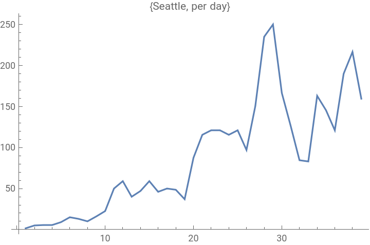
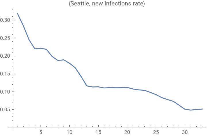
Both show some signs of stabilizing, with recent per-day new cases a bit lower than the peaks. Both have quotients around 0.07, and that gives some indication that my crude estimate might not be too far off. This is important in terms of calibrating this model.
Next we look at Chicago and Detroit.
Chicago and Detroit are both showing recent signs of improvement (five days ago they were still on the rise). And they both have quotients in the 0.10-0.11 range. The important thing, for them, is that these quotients are dropping. Moreover, if the Seattle and San Fran numbers continue to fall, the nice thing is that Chicago and Detroit are only between one and two weeks behind in terms of those quotients. San Francisco has been in an aggressive shelter-in-place for 3+ weeks now.
New York City has also been under a shelter-at-home order, and a bit longer than Illinois. But they may be affected by population density as well as more people going to-from the city despite the orders. Their quotient is just under 0.08, and dropping albeit not too fast of late. But they do seem to have recently crested. So that much is good. Five days ago the scenario was less clear, and more bleak.
And L.A. seems also to have turned back the tide in the past few days. The numbers suggest it is much better off than NYC (a factor of 10 fewer infections vs. approximately a factor of 2 smaller population). But this might just reflect that one region is doing more testing than another. Also I note that southern CA went into shelter-in-place at least a week after the Bay area. So it is plausible to expect a lag in terms of dropping the infection rate.
Florida notoriously delayed shelter-at-home until quite recently. Miami might be the hardest hit area. And it does seem to be quite sharply on the rise. It might not look steep, but recall the caveat about x-axes. This plot only covers but 28 days, vs. e.g. 70 for the City of Angels.
We now have a look at Dallas and Houston. As with Detroit, even averaging over 2-day spans did not do much to smooth the Dallas data (and with potential rapid rises I cannot justify larger-scale averaging). From the general look, not so bad. Numbers might be going up, or not, but they are not rising drastically. And that quotient is around 0.104. I show raw data beneath it by modifying the function slightly.
One will note that the number of new cases is not jumping hugely, and that infection rate quotient is indeed dropping.
Houston is not faring so well. Possibly related is that Dallas county issued shelter-in-place order on March 22, with the city following up (and that hits some other counties) on March 24. Houston issued a stay-at-home order on March 24. This appears to be a slightly weaker form of containment. That said, it is hard to know if such differences are behind the relatively worse situation for Houston, or whether it has to do with more accurate reporting of cases, or more cases due to other differences between the two regions.
Here are the three counties hardest hit (I believe) in New Jersey. All three remain in trouble it seems, although this should be more clear in another few days. Also all three are seeing a steady decline in the infection rate ratio, so that at least is a promising sign.
Here are New Orleans, Atlanta, Memphis and Denver, charted along with San Francisco and Seattle. New Orleans is a significantly smaller city than most of the others. This picture is not good for them, as of now.
Last I show a few of the largest cities, excepting New York, plotted together.
Summary
Summary
My goals was to simplify the infection model in a way that will apply to city-size regions under shelter-in-place orders. This gave us what I believe is a very important computable value: the quotient of new infections to current infections. The plots and numbers all point to the following: When that quotient gets below 0.1 or so, the numbers of new cases start to drop.
While this critical value may vary slightly from one location to another, it appears to occupy a fairly tight band. So, rather conveniently, it is close to scale-invariant, that is, (almost) independent of city size of population density.
Another very nice aspect is that this computation does not rely on full reporting of new cases; one can work directly with the official tallies and not be concerned with levels of under-reporting. This gives an easy measure of how well a given city is faring, along with the possibility of extrapolating the quotient to determine when the peak will hit and how large it might go.
Yet another feature is that it really makes no assumption about the particulars of the diesease (underlying cause, how spread, etc.) but only assumes that communities are minimizing their “contact surface”. So it might be useful should this virus rebound e.g. from seasonal effects, or should another jump the fence from animals to humans.