Uniquac Model for Water - iso-Butanol Binary Mixture at 1 atm
Housam Binous
Uniquac Model for Water - iso-Butanol Binary Mixture at 1 atm
Housam Binous
Housam Binous
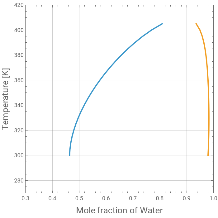
The code implements a full UNIQUAC liquid-liquid equilibrium (LLE) calculation for the binary system water (1) + isobutanol (2), using the binary interaction parameters extracted directly from Aspen Plus UNIQ-1 dataset. It proceeds in four stages: (1) define the UNIQUAC structural parameters (r, q) and the temperature-dependent τᵢⱼ(T) function from the Aspen Aᵢⱼ/Bᵢⱼ/Cᵢⱼ/Dᵢⱼ form; (2) build symbolic expressions for lnγ₁, lnγ₂, and the molar Gibbs energy of mixing Gmix/RT as explicit functions of composition x₁ and temperature T; (3) solve for the binodal (phase-split) compositions at each temperature via a common-tangent construction; and (4) sweep temperature to generate the full coexistence curve, which is then plotted twice — once in water mole fraction and once converted to mass fraction of isobutanol.
The τᵢⱼ function reproduces Aspen’s temperature form, ln(τᵢⱼ) = Aᵢⱼ + Bᵢⱼ/T + Cᵢⱼ·ln(T) + Dᵢⱼ·T, using the regressed values you pulled from the UNIQ-1 binary interaction table. The lnGamma1 and lnGamma2 functions implement the standard two-term UNIQUAC expression (combinatorial + residual contributions) using volume fractions φᵢ and area fractions θᵢ built from rPar = {0.92, 3.4535} and qPar = {1.40, 3.048}, with coordination number z = 10. These activity coefficients are combined into the molar excess Gibbs energy (GexRT) and then into the full Gmix/RT, which includes the ideal entropy-of-mixing term x₁ ln x₁ + x₂ ln x₂.
Phase-split solution method: Rather than directly equating activities in the two phases, the script locates the binodal by minimizing the Gibbs energy curve’s double-tangent line: it first finds the spinodal points (where d²G/dx² = 0) to get a bracketing initial guess, then uses FindRoot on a 2×2 nonlinear system enforcing equal slope (chemical potential) and equal tangent-line value at the two candidate compositions xₐ and xb. This is a more numerically robust approach than solving isoactivity equations directly, since the common-tangent formulation avoids convergence issues near the flat region of G(x) close to the critical point. The commonTangent[T] function returns {None, None} if no spinodal points exist (i.e., the system is predicted fully miscible at that T), which guards against failures as T approaches the consolute temperature.
Building and displaying the binodal curve. The script sweeps T from 300 K to 405 K in 5 K increments and tabulates the corresponding {xa, xb} pairs into the variable binodal. These are reshaped into two branches (t1 = water-rich, t2 = isobutanol-rich) and plotted as Temperature vs. mole fraction of water, giving a closed-loop coexistence curve typical of an upper critical solution temperature (UCST) system. The code then overlays the same plot with a Raster image (IMG) of literature/experimental data (see Ref. 1) for visual comparison between present UNIQUAC-predicted curve and real data.
Mass-fraction conversion and final comparison. In the final block, the code converts the binodal from mole fraction of water to mass fraction of isobutanol using MWisoButane = 74.12 g/mol and MWwater = 18 g/mol, producing a second plot with axes matching the classic Moriyoshi-style isobaric solubility diagram (Temperature on x-axis, mass fraction of i-butanol on y-axis). Both binodal plots are again overlaid with a digitized/rasterized image of literature data for direct visual validation (Ref. 2).
References:
[1] Winklbauer, L.; Qian, J.; Burger, J. “Vapor–liquid and liquid–liquid equilibrium in mixtures of water + isobutanol/n-butanol + isobutylal/n-butylal.” Fluid Phase Equilibria, 2025, 596, 114440. https://doi.org/10.1016/j.fluid.2025.114440
[2] Moriyoshi, T.; Aoki, Y.; Kamiyama, H. “Mutual solubility of i-butanol + water under high pressure.” Journal of Chemical Thermodynamics, 1977, 9 (5), 495–502. https://doi.org/10.1016/0021-9614(77)90151-3
(*UNIQUACmodelforLLE-systemiswater(1)+isobutanol(2)*)(*Structuralparameters*)rPar={0.9200,3.4535};qPar={1.400,3.048};
In[]:=
zCoord=10;
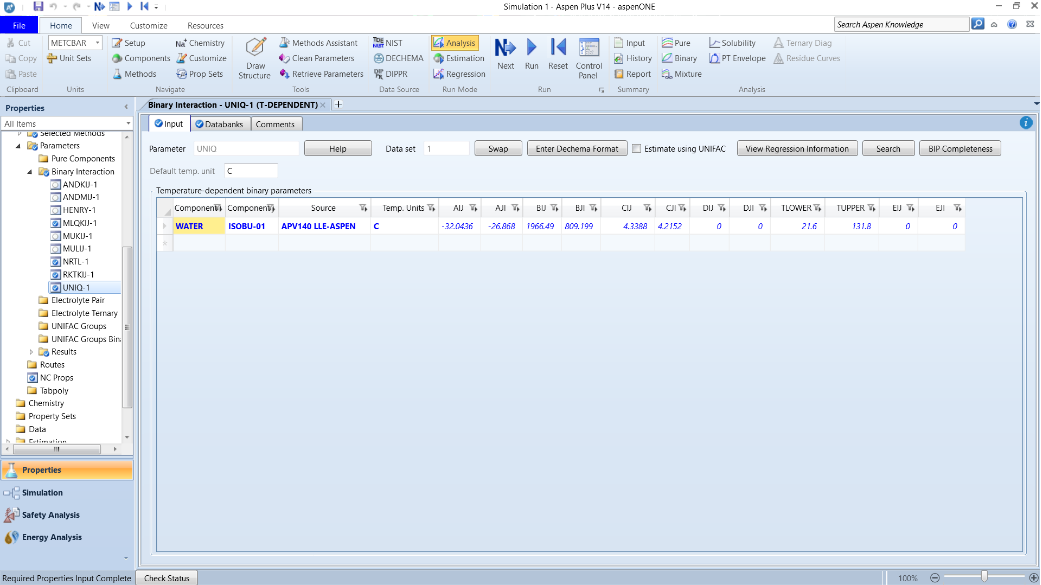
(*UNIQUACtau_ij(T)usingAspenPlusparameters*)(*ln(tau_ij)=Aij+Bij/T+Cij*Log[T]+Dij*T,Tlower=21.6°C<T<Tupper=131.8°C*)(*TinKelvin)*)(*BinaryparametersfromAspentable(Water=1,Isobutanol(ISOBU-01)=2)*)params=<|{1,2}-><|"A"->-32.0436,"B"->1966.49,"C"->4.3388,"D"->0,"Tlow"->21.6+273.15,"Thigh"->131.8+273.15|>,{2,1}-><|"A"->-26.868,"B"->809.199,"C"->4.2152,"D"->0,"Tlow"->21.6+273.15,"Thigh"->131.8+273.15|>|>;(*tau_ijattemperatureT(Kelvin)*)tauIJ[i_,j_,Tk_]:=Module[{p,lnTau},If[i==j,Return[1.0]];p=params[{i,j}];If[MissingQ[p],Return[0]];(*nodata->defineasneeded*)lnTau=p["A"]+p["B"]/Tk+p["C"]*Log[Tk]+p["D"]*Tk;Exp[lnTau]];(*Buildfullnxntaumatrixatagiventemperature*)tauMatrix[n_,Tk_]:=Table[tauIJ[i,j,Tk],{i,1,n},{j,1,n}];
In[]:=
(*ln(gamma1),ln(gamma2)asexplicitsymbolicfunctionsofx1,T*)lnGamma1[x1_,T_]:=Module[{x2,phi1,phi2,theta1,theta2,t12,t21},x2=1-x1;phi1=(x1*rPar[[1]])/(x1*rPar[[1]]+x2*rPar[[2]]);phi2=(x2*rPar[[2]])/(x1*rPar[[1]]+x2*rPar[[2]]);theta1=(x1*qPar[[1]])/(x1*qPar[[1]]+x2*qPar[[2]]);theta2=(x2*qPar[[2]])/(x1*qPar[[1]]+x2*qPar[[2]]);t12=tauIJ[1,2,T];t21=tauIJ[2,1,T];(Log[phi1/x1]+1-phi1/x1-(zCoord/2)*qPar[[1]]*(Log[phi1/theta1]+1-phi1/theta1))+qPar[[1]]*(1-Log[theta1+theta2*t21]-(theta1/(theta1+theta2*t21)+theta2*t12/(theta2+theta1*t12)))]lnGamma2[x1_,T_]:=Module[{x2,phi1,phi2,theta1,theta2,t12,t21},x2=1-x1;phi1=(x1*rPar[[1]])/(x1*rPar[[1]]+x2*rPar[[2]]);phi2=(x2*rPar[[2]])/(x1*rPar[[1]]+x2*rPar[[2]]);theta1=(x1*qPar[[1]])/(x1*qPar[[1]]+x2*qPar[[2]]);theta2=(x2*qPar[[2]])/(x1*qPar[[1]]+x2*qPar[[2]]);t12=tauIJ[1,2,T];t21=tauIJ[2,1,T];(Log[phi2/x2]+1-phi2/x2-(zCoord/2)*qPar[[2]]*(Log[phi2/theta2]+1-phi2/theta2))+qPar[[2]]*(1-Log[theta2+theta1*t12]-(theta2/(theta2+theta1*t12)+theta1*t21/(theta1+theta2*t21)))](*Gex/RT=x1ln(gamma1)+x2ln(gamma2)*)uniquacGexRT[x1_,T_]:=Module[{x2},x2=1-x1;x1*lnGamma1[x1,T]+x2*lnGamma2[x1,T]](*Gmix/RT=idealmixingentropy+excessterm*)gmixRT[x1_,T_]:=Module[{x2},x2=1-x1;x1*Log[x1]+x2*Log[x2]+uniquacGexRT[x1,T]](*Derivative(chemicalpotentialdifference)*)dgdx[x1_,T_]:=D[gmixRT[x,T],x]/.x->x1(*Spinodal:solved^2G/dx^2=0*)spinodalPoints[T_]:=Module[{d2g,sols},d2g=D[gmixRT[x,T],{x,2}];sols=x/.NSolve[{d2g==0,0<x<1},x,Reals];Sort[sols]](*Commontangent:solvethe2x2system(1)dG/dx|_xa=(G(xb)-G(xa))/(xb-xa)(2)dG/dx|_xb=(G(xb)-G(xa))/(xb-xa)*)commonTangent[T_]:=Module[{ga,gb,slope,eq1,eq2,guess,sol,xa,xb,sp},sp=spinodalPoints[T];If[Length[sp]<2,Return[{None,None}]];(*fullymiscible*)guess={sp[[1]]*0.5,sp[[-1]]+(1-sp[[-1]])*0.5};ga=gmixRT[xa,T];gb=gmixRT[xb,T];slope=(gb-ga)/(xb-xa);eq1=D[gmixRT[x,T],x]/.x->xa;eq2=D[gmixRT[x,T],x]/.x->xb;sol=FindRoot[{eq1-slope==0,eq2-slope==0},{{xa,guess[[1]]},{xb,guess[[2]]}},MaxIterations->2000,PrecisionGoal->20,AccuracyGoal->20];{xa,xb}/.sol]
In[]:=
(*Sweeptemperaturetobuildabinodalcurve*)Tvals=Range[300,405,5];binodal=Table[{T,commonTangent[T]},{T,Tvals}]
Out[]=
{{300,{0.46422,0.979654}},{305,{0.465493,0.980789}},{310,{0.468616,0.98164}},{315,{0.473402,0.982254}},{320,{0.479708,0.982663}},{325,{0.487426,0.982887}},{330,{0.496478,0.98294}},{335,{0.506807,0.982828}},{340,{0.518377,0.982551}},{345,{0.531169,0.982104}},{350,{0.545179,0.981473}},{355,{0.560419,0.980639}},{360,{0.576917,0.979571}},{365,{0.594721,0.978229}},{370,{0.613903,0.976554}},{375,{0.634563,0.97446}},{380,{0.656848,0.971826}},{385,{0.680975,0.968466}},{390,{0.707281,0.964079}},{395,{0.736337,0.958139}},{400,{0.769266,0.949578}},{405,{0.808997,0.935529}}}
In[]:=
t1=Table[{binodal[[i]][[2]][[1]],binodal[[i]][[1]]},{i,1,Length@binodal}];
In[]:=
t2=Table[{binodal[[i]][[2]][[2]],binodal[[i]][[1]]},{i,1,Length@binodal}];
In[]:=
p=ListPlot[{t1,t2},Joined->True,Frame->True,GridLines->Automatic,AspectRatio->1,ImageSize->350{1,1},PlotRange->{{0.3,1},{270,420}},FrameLabel->{Style["Mole fraction of Water",14],Style["Temperature [K]",14]}]
Out[]=