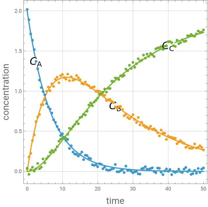
Consider two first-order, liquid-phase reactions ABC taking place in an isothermal batch reactor; the reactor initially contains only A at a concentration of 2 . The activation energy Ea2 of the second reaction (155 kJ/mol) is higher than the activation energy Ea1 of the first reaction (145 kJ/mol).The governing equations are:=-,=-,=,=, =,where , , and are the concentrations of , , and (), is time (h), and are the rate constants for the first and second reactions (1/h), and are pre-exponential factors (1/h), and are activation energies (kJ/mol) where <, is the ideal gas constant (kJ/[mol K]), and is temperature (K) of the reaction.Here, we generate hypothetical noisy data and use FindMinimum to determine the batch reactor’s temperature.
mol/
3
dm
C
A
t
k
1
C
A
d
C
B
dt
k
1
C
A
k
2
C
B
d
C
C
dt
k
2
C
B
k
1
A
1
-
Ea
1
RT
e
k
2
A
2
-
Ea
2
RT
e
C
A
C
B
C
C
A
B
C
mol/
3
dm
t
k
1
k
2
A
1
A
2
Ea
1
Ea
2
Ea
1
Ea
2
R
T
In[]:=
Clear[T]
Rate constants
Ea1=145;Ea2=155;R=8.314*^-3;A1=3.6*^16;A2=1.8*^17;k1=A1*Exp-;k2=A2*Exp-;
Ea1
R*T
Ea2
R*T
Initial concentration
Cao=2.0;
Temperature
T=435.85;
Solution of ODEs at T = 435.85
sol=Quiet@NDSolve[{Ca'[t]-k1*Ca[t],Cb'[t]k1*Ca[t]-k2*Cb[t],Cc'[t]k2*Cb[t],Ca[0]Cao,Cb[0]0,Cc[0]0},{Ca,Cb,Cc},{t,0,50}][[1]];
p1=Show[Plot[{Ca[t]/.sol,Cb[t]/.sol,Cc[t]/.sol},{t,0,50},PlotStyleThick,PlotRangeAll],Graphics@Text[Style[Subscript[Style["C",Italic],"A"],18,Black,BackgroundWhite],{0.05*50,Ca[0.05*50]/.sol}],Graphics@Text[Style[Subscript[Style["C",Italic],"B"],18,Black,BackgroundWhite],{0.5*50,Cb[0.5*50]/.sol}],Graphics@Text[Style[Subscript[Style["C",Italic],"C"],18,Black,BackgroundWhite],{0.8*50,Cc[0.8*50]/.sol}]];
Generating noisy data to mimic experimental data with some noise
In[]:=
SeedRandom[1234]
Out[]=
RandomGeneratorState
In[]:=
tbl1=Table[{t,Evaluate[Ca[t]/.sol]+0.05(2Random[]-1)},{t,0,50,0.5}];tbl2=Table[{t,Evaluate[Cb[t]/.sol]+0.05(2Random[]-1)},{t,0,50,0.5}];tbl3=Table[{t,Evaluate[Cc[t]/.sol]+0.05(2Random[]-1)},{t,0,50,0.5}];
In[]:=
data=Join[{{Style["time ",Red],Style["A",Red],Style["B",Red],Style["C",Red]}},Table[{tbl1[[i]][[1]],tbl1[[i]][[2]],tbl2[[i]][[2]],tbl3[[i]][[2]]},{i,1,Length@tbl1,4}]]//TableForm
Out[]//TableForm=
time | A | B | C |
0. | 2.01812 | 0.0306518 | 0.0395539 |
2. | 1.5186 | 0.455484 | 0.00465467 |
4. | 1.04569 | 0.831159 | 0.0526821 |
6. | 0.802847 | 1.05132 | 0.187839 |
8. | 0.613396 | 1.14773 | 0.267773 |
10. | 0.469967 | 1.2083 | 0.415441 |
12. | 0.286531 | 1.13111 | 0.53774 |
14. | 0.212213 | 1.1954 | 0.619039 |
16. | 0.148009 | 1.08645 | 0.712656 |
18. | 0.158251 | 1.04246 | 0.854404 |
20. | 0.0593851 | 1.00386 | 0.912964 |
22. | 0.0570553 | 0.94809 | 1.02736 |
24. | 0.029491 | 0.872573 | 1.12506 |
26. | -0.00414939 | 0.808662 | 1.14596 |
28. | 0.0669382 | 0.71187 | 1.27455 |
30. | -0.0162151 | 0.706333 | 1.35813 |
32. | -0.0330536 | 0.580554 | 1.37453 |
34. | 0.0283568 | 0.549006 | 1.46216 |
36. | -0.000483662 | 0.531072 | 1.43182 |
38. | -0.00886303 | 0.516369 | 1.55443 |
40. | 0.00191979 | 0.440036 | 1.61662 |
42. | -0.0113571 | 0.413721 | 1.55797 |
44. | -0.0131318 | 0.360932 | 1.6405 |
46. | 0.0197354 | 0.290871 | 1.68817 |
48. | -0.0214775 | 0.293389 | 1.71446 |
50. | 0.0435284 | 0.268661 | 1.76225 |
Exact data vs. noisy data
In[]:=
Show[p1,ListPlot[{tbl1,tbl2,tbl3},PlotStyle->PointSize[0.015]],FrameLabel->{Style["time",16],Style["concentration",16]},Frame->True,AspectRatio->1,GridLines->Automatic]
Out[]=
We propose to fetch the temperature of the batch reactor
T=.
In[]:=
solt[T_?NumericQ]:=NDSolve[{Ca'[t]-k1*Ca[t],Cb'[t]k1*Ca[t]-k2*Cb[t],Cc'[t]k2*Cb[t],Ca[0]Cao,Cb[0]0,Cc[0]0},{Ca,Cb,Cc},{t,0,50}][[1]]
In[]:=
MYOBJ[T_?NumericQ]:=Sum[Evaluate[(tbl1[[i]][[2]]-Ca[tbl1[[i]][[1]]])^2+(tbl2[[i]][[2]]-Cb[tbl1[[i]][[1]]])^2+(tbl3[[i]][[2]]-Cc[tbl1[[i]][[1]]])^2]/.solt[T],{i,1,Length@tbl1}]
We minimize the sum of the squared deviations --- we find T=435.862 K close to the ideal situation or noise-free case where T=435.85 K
In[]:=
FindMinimum[MYOBJ[T],{T,430},Method->"InteriorPoint"]
Out[]=
{0.238148,{T435.862}}
Determination of kinetic parameters from experimental concentrations
Determination of kinetic parameters from experimental concentrations
We propose to fetch the kinetic parameters
Clear[Ea1,Ea2,A1,A2]
In[]:=
solt[Ea1_?NumericQ,Ea2_?NumericQ,A1_?NumericQ,A2_?NumericQ]:=NDSolve[{Ca'[t]-k1*Ca[t],Cb'[t]k1*Ca[t]-k2*Cb[t],Cc'[t]k2*Cb[t],Ca[0]Cao,Cb[0]0,Cc[0]0},{Ca,Cb,Cc},{t,0,50}][[1]]
In[]:=
MYOBJ[Ea1_?NumericQ,Ea2_?NumericQ,A1_?NumericQ,A2_?NumericQ]:=Sum[Evaluate[(tbl1[[i]][[2]]-Ca[tbl1[[i]][[1]]])^2+(tbl2[[i]][[2]]-Cb[tbl1[[i]][[1]]])^2+(tbl3[[i]][[2]]-Cc[tbl1[[i]][[1]]])^2]/.solt[Ea1,Ea2,A1,A2],{i,1,Length@tbl1}]
We minimize the sum of the squared deviations --- we find: Ea1=145.084, Ea2=154.915, A1=3.6965, A2=1.7567
In[]:=
Clear[Ea1,Ea2,A1,A2]
In[]:=
FindMinimum[{MYOBJ[Ea1,Ea2,A1,A2],A1>=3.5,A2>=1.75},{Ea1,140},{Ea2,150},{A1,3},{A2,2},Method->"InteriorPoint"]
Out[]=
{0.0593434,{Ea1145.084,Ea2154.915,A13.69659,A21.75673}}
References
References
[1] This notebook builds on the following demonstration: https://demonstrations.wolfram.com/SeriesReactionsInABatchReactor/
CITE THIS NOTEBOOK
CITE THIS NOTEBOOK
Temperature determination from concentration data for series reactions in a batch reactor
by Housam Binous and Ahmed Bellagi
Wolfram Community, STAFF PICKS, October 6, 2025
https://community.wolfram.com/groups/-/m/t/3557081
by Housam Binous and Ahmed Bellagi
Wolfram Community, STAFF PICKS, October 6, 2025
https://community.wolfram.com/groups/-/m/t/3557081