Exponential decay of time in a Wolfram model given by a string substitution system

Contributor: José Manuel Rodríguez Caballero

Update: March 12, 2021

Abstract

In the framework of the Wolfram Model, we study a string substitution system where the macroscopic time is related to the microscopic time via exponential decay.

Toy universe

In the framework of the Wolfram Model, we develop a toy universe, where space is a string substitution system.
https://www.wolframphysics.org/technical-introduction/the-updating-process-for-string-substitution-systems/string-substitution-systems/

In this toy model, macroscopic time (time measured by a clock) is related to microscopic time (number of elementary operations performed in the universe) through the exponential decay formula. This notion of microscopic time corresponds to the time in the Wolfram Model (we are adding “microscopic” just to distinguish it from the other notion of time).
https://www.wolframphysics.org/technical-introduction/potential-relation-to-physics/time-and-spacetime/

State

Let n be a positive integer. We consider a toy universe consisting of a string of length n, where each character is A, B, or C. This string is analogous to the spatial hypergraph in the Wolfram model, i.e., space (not to be confused with spacetime).

Hypothesis about the observer

We assume that any observer in our toy universe can distinguish B from either A or C, but it cannot distinguish between A and C.

Initial condition

As initial condition, we will assume a uniform distribution in the list, where the frequency of A, B, C are 1/4, 1/2, 1/4 respectively.

In[]:=

InitialCondition[n_]:=StringJoin[Table[RandomChoice[{0.25,0.5,0.25}{"A","B","C"}],{n}]]

Example of initial condition.

In[]:=

InitialCondition[60]

Out[]=

BABBCAABBBBBBAABABBBCABBBBAABBCAABABBBCBABBBBCCAABBBBABCBBBB

Evolution

At any time, choose a random position in the list and apply the transformations:

if the element at this position is B, rewrite it as A;

if the element at this position is A, rewrite it as C;

if the element at this position is C, rewrite it as A.

Graphically:

In[]:=

Graph[{"B""A","A""C","C""A"}]

Out[]=

In[]:=

Evolution[s_(*state*),t_(*time*)]:=ResourceFunction["SubstitutionSystemCausalEvolution"][{"B""A","A""C","C""A"},s,t,"Random"]

Example of evolution.

In[]:=

Evolution[InitialCondition[60],10]//TableForm

Out[]//TableForm=

CBABCACBBCACBBBBBBABCBBCABBCBCBBBBBAABCBBABBCBCBACBBBBBBABCB

CBABCACBBCACBBBBBBABCBBCABBCBCBABBBAABCBBABBCBCBACBBBBBBABCB

{32,32}{32,32}

CBABCACBBCACBBBBBBABCBBCABBCBCBABBBAABCBBABACBCBACBBBBBBABCB

{44,44}{44,44}

CBABCACBBCACBBBBBBABCBBCABBCBCBABBBAABCBBABACBCAACBBBBBBABCB

{48,48}{48,48}

CBABCACBBCACBBBBBBABCBBCABBCBCBABBBAABCBBCBACBCAACBBBBBBABCB

{42,42}{42,42}

CBABCACBBCACBBBBBBABCBBCABBCBCBABBBAABCBBCAACBCAACBBBBBBABCB

{43,43}{43,43}

CBABCACBBCACBBBBBBABCBBCABBCBCBABBBAABCBBCAAABCAACBBBBBBABCB

{45,45}{45,45}

CBABCACBBCACBBBBBBABCBBCABBCBCBABBBAABCBBCAAABCAACBBBBBAABCB

{56,56}{56,56}

CBABCACBBCACBBBBBBABCBBCABBCBCBABBBAABCBBCAAABCAACBABBBAABCB

{52,52}{52,52}

CBABCACBBCAABBBBBBABCBBCABBCBCBABBBAABCBBCAAABCAACBABBBAABCB

{12,12}{12,12}

CBABCACBBCCABBBBBBABCBBCABBCBCBABBBAABCBBCAAABCAACBABBBAABCB

{11,11}{11,11}

Spacetime

We will use the causal graph to represent spacetime of this Wolfram Model.
https://www.wolframphysics.org/technical-introduction/the-updating-process-for-string-substitution-systems/events-and-their-causal-relationships/

In[]:=

Spacetime[s_(*state*),t_(*time*)]:=ResourceFunction["MultiwaySystem"][{"B"->"A","A"->"C","C"->"A"},s,t,"CausalGraphStructure",VertexLabelsNone]

In[]:=

Spacetime[InitialCondition[10],4]

Out[]=

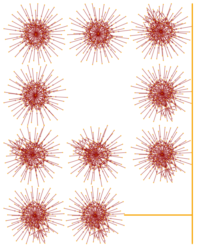
Remark: This space-time structure resembles G. t’Hooft’s explanation of the holographic principle: due to loss of information, the interior of a region disappears and all information is stored at the boundary. https://arxiv.org/pdf/2005.06374.pdf

Quantum structure

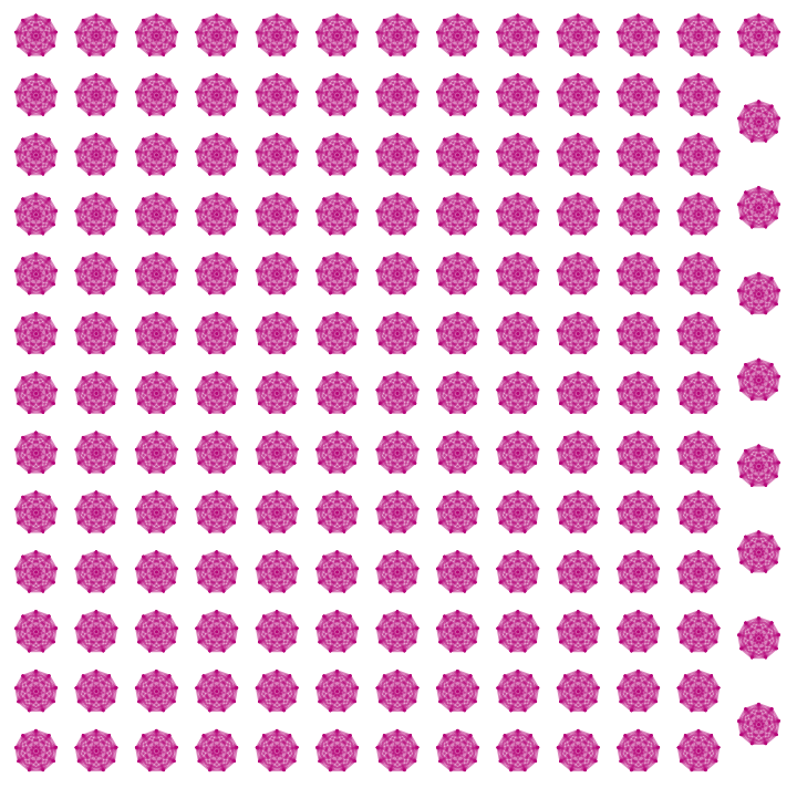
We will use the branchial space to represent quantum properties of this Wolfram Model.
https://www.wolframphysics.org/technical-introduction/the-updating-process-for-string-substitution-systems/the-concept-of-branchial-graphs/

In[]:=

QuantumEntanglement[s_(*state*),t_(*time*)]:=ResourceFunction["MultiwaySystem"][{"B"->"A","A"->"C","C"->"A"},s,t,"EventBranchialGraphStructure"]

In[]:=

QuantumEntanglement[InitialCondition[10],4]

Out[]=

Macroscopic time

Formula in the continuous approximation

We define the microscopic time of our toy universe, denoted τ, as the number of elementary computational operations divided by the size of space (length of the string). Notice that microscopic time can be as large as we want.

We define the macroscopic time of our toy universe, denoted t, the density both A and C minus the density of B, all divided by the size of space (length of the string). This definition is motivated by the hypothesis about the observed formulated above, i.e., any observer in our toy universe can distinguish B from either A or C, but it cannot distinguish between A and C. A clock in this universe is a machine that measures the density of (A or C) and the density of B. Notice that macroscopic time is bounded between 0 and 1.

In[]:=

t[s_]:=N[StringCount[s,"A"]+StringCount[s,"C"]-StringCount[s,"B"]]/StringLength[s]

The relationship between macroscopic and microscopic time can be derived from the differential equation

dt/dτ = 1 - t (differential equation)

Solving this problem

In[]:=

DSolve[{T'[τ]1-T[τ],T[0]μ},T[τ],τ]//FullSimplify

Out[]=

{{T[τ]1+

-τ



(-1+μ)}}

we conclude that the macroscopic time is in exponential decay with respect to the microscopic time, i.e.,

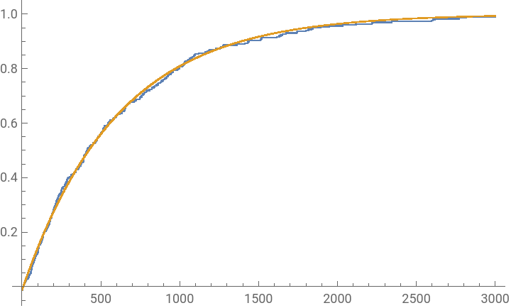
t = 1 - (1 - μ) * Exp[ -τ ].

where μ is the macroscopic time of the initial condition.

Experimental verification

In[]:=

n=600;(*sizeofspace*)L=First/@Evolution[InitialCondition[n],3000(*numberofsteps*)];c=1-t[L[[1]]];ListPlot[{Table[t[L[[i]]],{i,#}],Table[1-c*Exp[-i/n],{i,#}]}]&[Length[L]]

Out[]=

Shannon entropy of the toy universe as a function of macroscopic time.

H(t) = h*( -(1 + t)/2*Log[2, (1 + t)/2] - (1 - t)/2*Log[2, (1 - t)/2] )

where h is the initial entropy.

Experimental verification

We already attempted to explain beta decay by following Bohr’s approach rather than Pauli’s.
https://community.wolfram.com/groups/-/m/t/2214823

Conjecture (Bohr). During beta-decay, there is a violation of the conservation of energy.

Notice that our toy universe is invariance under time translations if and only if there are no characters B.

Applying Noether’s theorem (it makes no sense, this is just a heuristic analogy), we conclude that during all its history (from t = 0 to t = 1), there is no conservation of energy in our toy universe.

Therefore, at least in our toy universe, the violation of the conservation of energy is correlated to the emergence of (macroscopic) time.

Future work

We hope that some of the ideas presented in this essay can be extended from this string substitution system to a hypergraph model.

To continue the search of Wolfram models related to beta decay.