Fluid flow analysis through squared arrangements of pipes
by Giuseppe Parasiliti Rantone
Institut Jean Le Rond d’Alembert, Sorbonne Université and the company Gaztransport & Technigaz (GTT)
by Giuseppe Parasiliti Rantone
Institut Jean Le Rond d’Alembert, Sorbonne Université and the company Gaztransport & Technigaz (GTT)
The main goal is to study fluid flow through a closed arrangement of pipes using the finite elements method. The equations we take into consideration are Navier-Stokes equations eventually coupled with the energy conservation equation. We study the behaviour of laminar flows on different types of meshes, we start from a simple two dimensional mesh, we then extend the analysis to the Sierpinski carpet and the Menger Sponge. Sierpinski carpet is a two dimensional mesh that iteration by iteration assume fractal patterns, the Menger Sponge is its three dimensional extension. We deal with different boundary conditions, we impose both pressure and temperature gradients between the walls. We study both stationary and unsteady problems. We find several flow patterns and we understand how laminar flow behaves on fractal meshes and how boundary conditions are crucial to this behaviour. Next steps will be to extend the analysis to turbulent flows and to make an unsteady analysis of the stationary flows we considered.
Introduction
Introduction
Fluid flows are natural processes we experiment in our everyday life and despite that, their features are still partly unknown. Fluid motion is the result of viscous forces, pressure variations and gravitational forces. Given some initial condition and some boundary constraints, the equations fluids are governed by are called Navier-Stokes equations. They consist in the mass and the momentum conservation laws :ρ+∇(ρu)=0,(ρu)+∇(ρuu)+∇p=∇·σ+ρg.Where ρ is the density of the fluid, is the velocity, is the pressure, is the gravity and the stress tensor. The unknowns are the velocity and pressure all over the domain.Navier-Stokes equations could be coupled with the energy conservation equation, introducing the temperature as additional unknown of the flow. This equation reads:.Where is the specific heat at constant pressure, is a thermodynamic parameter, is the symmetric part of the Jacobian of velocity and is the heat conduction coefficient.The aim of the following is to study the behaviour of a fluid flow on domains with particular features. We will study both pressure and temperature-controlled laminar flows. This means that we will impose different values of pressure ( temperature) at the boundary of the domain and we will analyze the resulting flow patterns. We will take in consideration different types of domains. We will start with the study of a two dimensional squared arrangement of pipes, then we will handle fractal meshes. They have the feature that they show the same pattern at different scales. We will take into consideration the two dimensional Sierpinski carpet for different iterations and then its three dimensional extension, the Menger Sponge.
∂
t
∂
t
u
p
g
σ
ρ(T+u∇T)=α(p+u∇p)+σ:D(u)-∇·(k∇T)
C
p
∂
t
∂
t
C
p
α
D(u)
k
Pressure-controlled laminar flows
Pressure-controlled laminar flows
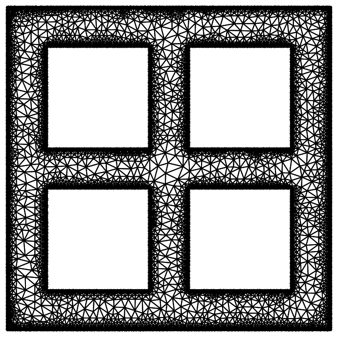
Let us construct a symmetric squared arrangement of pipes. Notice that the domain is constructed as a Region and that the function we decided to use for refinement is MaxBoundaryCellMeasure.
L=3;=L/4;=L/4;α=Rectangle[{0,0},{L,L}];=Rectangle[{/2,/2},{7*/4,7*/4}];=Rectangle[{/2,/4+L/2},{7*/4,6*/4+L/2}];=Rectangle[{/4+L/2,/2},{3*/2+L/2,7*/4}];=Rectangle[{/4+L/2,/4+L/2},{3*/2+L/2,3*/2+L/2}];Κ=RegionUnion[,,,];ω=RegionDifference[α,Κ];mesh=ToElementMesh[ω,"MaxBoundaryCellMeasure"->0.005,"MeshElementType"->TriangleElement];mesh["Wireframe"]
x
1
y
1
β
1
x
1
y
1
x
1
y
1
β
2
x
1
y
1
x
1
y
1
β
3
x
1
y
1
x
1
y
1
β
4
x
1
y
1
x
1
y
1
β
1
β
2
β
3
β
4
Let us assume that the density of the flow is constant and that gravity could be neglected. The Navier-Stokes equations for two dimensional domains reduce to the following:Where have introduced the kinematic viscosity . Let us set and We had some issues in the full finite elements analysis with NDSolve, that’s why we decided to perform a semi-discretization in time, by remaining partially explicit in treating the non linear terms and completely implicit for the other linear terms. The equations become:Let us fix a time step dt and construct the time independent operator as follows:
ρ(u+uu+vu)+p=μ(u+u),ρ(v+uv+vv)+p=μ(v+v),u+v=0.
∂
t
∂
x
∂
y
∂
x
∂
x,x
∂
y,y
∂
t
∂
x
∂
y
∂
y
∂
x,x
∂
y,y
∂
x
∂
y
μ
ρ=1
μ=.
-4
10
ρ-+++=μ+,ρ-+++=μ+,+=0.
n+1
u
n
u
Δt
n
u
∂
x
n+1
u
n
v
∂
y
n+1
u
∂
x
n+1
p
∂
x,x
n+1
u
∂
y,y
n+1
u
n+1
v
n
v
Δt
n
u
∂
x
n+1
v
n
v
∂
y
n+1
v
∂
y
n+1
p
∂
x,x
n+1
v
∂
y,y
n+1
v
∂
x
n+1
u
∂
y
n+1
v
In[]:=
dt=0.02;op1[i_]={ρ((u[x,y]-xVel[i-1][x,y])/dt+xVel[i-1][x,y]u[x,y]+yVel[i-1][x,y]u[x,y])-μ(u[x,y]+u[x,y])+p[x,y]==0,ρ((v[x,y]-yVel[i-1][x,y])/dt+xVel[i-1][x,y]v[x,y]+yVel[i-1][x,y]v[x,y])-μ(v[x,y]+v[x,y])+p[x,y]==0,u[x,y]+v[x,y]==0}/.{ρ->1,μ->};
∂
x
∂
y
∂
x,x
∂
y,y
∂
x
∂
x
∂
y
∂
x,x
∂
y,y
∂
y
∂
x
∂
y
-4
10
Let us give time independent boundary conditions for closed domains by imposing a pressure gradient between the walls and no-slip conditions for velocity on all boundary edges:
boundaryconditions1={DirichletCondition[{u[x,y]==0.,v[x,y]==0.},True],DirichletCondition[p[x,y]==0,x==L],DirichletCondition[p[x,y]==1,x==0]};
Let us give some initial conditions and create a time loop in which at each time step we solve Navier-Stokes equations in space on the squared arrangement of pipes. We will use a finite elements method with a quadratic order of interpolation for velocity and a linear order for pressure.
xVel[0][x_,y_]:=0;yVel[0][x_,y_]:=0;pressure[0][x_,y_]:=0;Table[{xVel[i],yVel[i],pressure[i]}=NDSolveValue[{op1[i],boundaryconditions1},{u,v,p},{x,y}∈mesh,Method->{"FiniteElement","InterpolationOrder"->{u->2,v->2,p->1}}],{i,1,15}];
Let us show the flow:
In[]:=
StreamPlot[{xVel[currenttime][x,y],yVel[currenttime][x,y]},{x,y}∈xVel[currenttime]["ElementMesh"],AspectRatio->Automatic,PlotRange->All,PlotLegendsAutomatic,ImageSize->Medium]
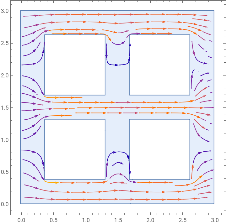

From the StreamPlot we see that the horizontal velocity is practically zero in the vertical pipes and that the flow is completely horizontal. Moreover the fluid flows in opposite direction of the gradient of pressure accordingly to what could be predictable a priori.
Let us show the values of Reynolds number in both x and y directions to confirm that we are in laminar flow.
{minX,maxX}=MinMax[xVel[currenttime]["ValuesOnGrid"]];{minY,maxY}=MinMax[yVel[currenttime]["ValuesOnGrid"]];characteristicUx=(Abs[minX]+Abs[maxX])/2;characteristicUy=(Abs[minY]+Abs[maxY])/2;ReynoldsX={ρUL/μ}/.{μ->,ρ->1,U->characteristicUx}ReynoldsY={ρUL/μ}/.{μ->,ρ->1,U->characteristicUy}
-4
10
-4
10
Out[]=
{2981.81}
Out[]=
{5711.32}
Let us now deal with more complex boundary conditions, we will impose the pressure to be in the left and top walls, in the right and bottom ones:
1
0
In this case a StreamPlot of component of velocities at the last time gives the following:
An animation of the ContourPlot of the module of velocity for each time step follows:
We notice that the flow is diagonal as we could expect.
The StreamPlot of components of velocity gives:
Notice that we obtain a result very similar to the first simulation, the flow is still horizontal, but here we have that velocity has higher values, especially at the left border where now is no more null.
Temperature-controlled laminar flows
Temperature-controlled laminar flows
Let us give boundary conditions for closed domains by imposing a temperature gradient between the walls, no-slip conditions for velocity on all boundary edges and a value for pressure in a point of the boundary:
We will solve full Navier-Stokes equations through NDSolve. Let us use the Monitor function to control that times go on without problems during the computation. The structure of NDSolve is similar to the previous cases, we just enrich the Method Option.
The ContourPlots of pressure and temperature give the following:
The StreamPlot of component of velocities gives:
The Sierpinski carpet
The Sierpinski carpet
Let us now construct a different type of meshes: the Sierpinski Carpet. They are created by iteration:
◼
at iteration 1 the square is divided in a grid of nine squares and the central square is removed;
◼
at iteration 2 the same procedure of the previous iteration is applied to every one of the eight remaining square and so on.
In Mathematica there is a function MengerMesh that takes in input the number of iterations and the dimension, that in two dimensions creates the Sierpinski carpet.
Let us take the pressure-controlled flow’s operator with the same initial and boundary conditions of the first simulation. The StreamPlots for the first three orders of iteration at final time give:
If we take the temperature-controlled flow’s operator with the same initial and boundary conditions of the stationary simulation previously performed, the VectorPlots and StreamPlots for the first three orders of iteration give:
The Menger sponge
The Menger sponge
The Menger Sponge is the three dimensional version of the Sierpinski carpet. The way it is constructed is the extension to one more dimension of the one we have explained in the previous section. We have created the mesh with the same function as before but in dimension 3.
Let us give the same boundary conditions of the first simulation extended to three dimensions, so no-slip boundary conditions for the three components of velocity and gradient of pressure between two walls (that now are surfaces and no more lines):
The solver also is an extension of the previous:
What we obtain by performing a StreamPlot3D with the components of velocity is the following:
Notice that what we obtain is exactly the extension of what we obtained previously. The comments on flow and patterns are the same of the two dimensional simulation. Here we notice that we have a flow on every face but the two faces where we impose pressure, as expected.
Conclusions and future Perspectives
Conclusions and future Perspectives
In this work we have studied the laminar flow of a fluid governed by Navier-Stokes equations , eventually coupled with the energy equation, with different boundary conditions. We have studied different meshes in different dimensions and we have observed flow patterns and features. In pressure-driven flows we have the generation of flows that have same direction and opposite bearing with respect to the pressure gradient, while in temperature-driven flows we have the generation of a circular flow. Moreover we have understood what is the behaviour of fractal meshes with respect to the laminarity of the flow. In pressure-driven flows the bigger is the iteration the bigger is Reynolds number, meaning that by increasing the order of iteration we make the flow tend to be turbulent. In temperature-driven flows the bigger is the iteration the lower is Reynolds number, meaning that by increasing the order of iteration we make the flow more and more laminar.
We would like to extend our analysis in order to be more representative of the different boundary and initial conditions possible as well as study the flow patterns appearing in open domains. A further refinement of the fractal domain flow to meshes corresponding to more iterations of the fractal construction process is also of high interest to us.
Keywords
Keywords
◼
Fluid Dynamics
◼
Laminar Flow
◼
Sierpinski Carpet
◼
Menger Mesh
◼
Finite Element Method
Acknowledgment
Acknowledgment
My sincere thanks to Sotiris who accompanied me on this adventure. Despite the thousands of difficulties, he managed to always be by my side and support me whenever I needed it. Thanks to Oliver who helped me a lot on understanding the weak points of my project. Thanks to Swastik who helped me with the debugging. Thanks to every person I had the opportunity to meet and with whom to discuss and learn new things. Thanks to Mads,Danielle, Emily and everyone who contributed to the organisation of the Summer School. Thanks to Stephen for having made this an unique experience.
References
References