The Samuelson multiplier-accelerator model is a classic dynamical account of the business cycle, in which consumption () responds to past income (ℐ) and investment (ℐ) responds to the change in income (Δℐ). This example takes that abstract model and grounds it in reality: we import postwar US national-accounts data from the St. Louis Federal Reserve’s public economic database (FRED), estimate the model’s two behavioral parameters directly from the data, and simulate the economy’s response. The result shows that a simple model from 1939, fit to eight decades of real data, reproduces the actual quarter-to-quarter swings in US GDP — capturing everything from ordinary cycles to the 2020 pandemic shock.
"𝒞𝒮" | "Consumption" |
"ℐ𝒱" | "Investment" |
"𝒢ℰ" | "Government expenditure (autonomous)" |
"𝒞𝒮" "a" | "Autonomous consumption" |
"ℐ𝒱" "a" | "Autonomous investment" |
"α" | "Marginal propensity to consume — multiplier 1/(1−α)" |
"β" | "Accelerator — induced investment per unit Δ income" |
"k" | "Discrete time index (quarters)" |
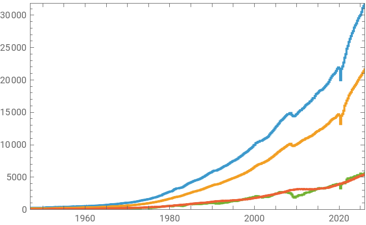
Import quarterly income (GDP ℐ), consumption (PCEC ), investment (GPDI ℐ), and government spending (GCE->ℰ) from FRED:
In[]:=
Import["https://fred.stlouisfed.org/graph/fredgraph.csv?id=GDP,PCEC,GPDI,GCE","Tabular"];data=RenameColumns[%,{"GDP"->"ℐ","PCEC"->"","GPDI"->"ℐ","GCE"->"ℰ"}]
Out[]=
Tabular


Extract each column from the table as a plain list of values:
In[]:=
ListStepPlotTable[data->{"observation_date",col},{col,{"ℐ","","ℐ","ℰ"}}],
Out[]=


Take quarter-to-quarter changes to strip out the long-run growth trend:
In[]:=
dataΔ=TransformColumns[data,Table[With[{c=col},"Δ"<>c->(ColumnwiseThread[Prepend[Differences[Slot[c]],0]]&)],{col,{"ℐ","","ℐ","ℰ"}}]]
Out[]=
Tabular
The Samuelson economic model:
In[]:=
Columneqns={ℐ[k]==[k]+ℐ[k]-ℰ[k],[k]==[k]+αℐ[k-1],ℐ[k]==ℐ[k]+β(ℐ[k-1]-ℐ[k-2])},
Out[]=
ℐ[k][k]-ℰ[k]+ℐ[k] |
[k][k]+αℐ[-1+k] |
ℐ[k]ℐ[k]+β(-ℐ[-2+k]+ℐ[-1+k]) |
Fitting the model's two behavioral equations, in differenced form (differencing cancels the unobserved autonomous terms and the shared trend):
Δ[k] = const + α·Δℐ[k-1]
Δℐ[k] = const + β·Δ²ℐ[k-1]
Δ[k] = const + α·Δℐ[k-1]
Δℐ[k] = const + β·Δ²ℐ[k-1]
In[]:=
{Δℐ,Δ,Δℐ,Δℰ}=Table[dataΔ[[All,col]],{col,ColumnKeys[dataΔ][[{6,7,8,9}]]}];
α: regress ΔC[k] on ΔNI[k-1], with intercept (intercept = autonomous-drift diagnostic, not a validity check).
In[]:=
α=Coefficient[Fit[({Δℐ[[2;;-2]],Δ[[3;;]]}),{1,x},x],x]
Out[]=
0.131391
β: regress ΔI[k] on Δ²NI[k-1] = ΔNI[k-1]−ΔNI[k-2]. The k-1 lag matters — using k instead flips β's sign.
In[]:=
β=Coefficient[Fit[{Differences[Δℐ][[;;-2]],Δℐ[[3;;]]},{1,x},x],x]
Out[]=
-0.00836656
Assemble the model’s input data from the trend-free data:
In[]:=
ℰ
tfDat
In[]:=
tfDat
In[]:=
ℐ
tfDat
In[]:=
inpSig={,,}
ℰ
tfDat
tfDat
ℐ
tfDat
Out[]=
TabularColumn,TabularColumn,TabularColumn
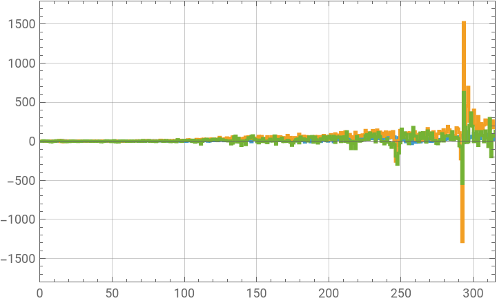
Plot the model’s three driving inputs each a bounded fluctuation once the trend its trend is removed:
In[]:=
ListStepPlotinpSig,
Out[]=
The state space model:
In[]:=
ssm=StateSpaceModel[eqns,{ℐ[k],[k],ℐ[k]},{ℰ[k],[k],ℐ[k]},{ℐ[k]},k]
Out[]=
0.1230 | 0.0084 | 1.0000 | -1.0000 | -1.0000 |
1.0000 | 0.0000 | 0.0000 | 0.0000 | 0.0000 |
-0.1230 | -0.0084 | -1.0000 | 1.0000 | 1.0000 |
1
Drive the model using the input signal:
In[]:=
or=OutputResponse[ssm,inpSig][[1]];
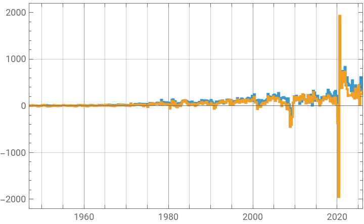
The model replicates ℐ fluctuations with accurately with the largest being the 2020 COVID crash and subsequent recovery:
In[]:=
dataΔM=InsertColumns[dataΔ,"model"->PadLeft[or,Length[dataΔ]]];
In[]:=
ListStepPlotTable[dataΔM->{"observation_date",col},{col,{"Δℐ","model"}}],
Out[]=
CITE THIS NOTEBOOK
CITE THIS NOTEBOOK
Samuelson economic model with real GDP data
by Maher Kuzbari
Wolfram Community, STAFF PICKS, July 10, 2026
https://community.wolfram.com/groups/-/m/t/3755722
by Maher Kuzbari
Wolfram Community, STAFF PICKS, July 10, 2026
https://community.wolfram.com/groups/-/m/t/3755722