Author's note. This project was primarily an experiment to see how far a current LLM (Claude Code, model Opus 4.7 with the 1 M-token context window) can get in the Wolfram Language with very little human guidance. I supplied the target -- 'render a Kerr black hole with a real lensed sky and a physically motivated accretion disk, package it as a Wolfram Community post' -- and a handful of correction nudges (e.g. 'put a recognisable galaxy behind the BH', 'centre the figures', 'check that escaped rays actually sample the panorama'). Everything else, including the Hamiltonian geodesic integrator, the Bardeen-impact-parameter machinery, the Novikov-Thorne disk model, the equirectangular sky compositor and the RemoteBatchSubmit pipeline, was written by the model. All Kerr renders, the characteristic-radii plot and the equirectangular sky panorama in this notebook are produced in pure Wolfram Language by the included build_realistic_sky.wls and render_assets.wls scripts (and the included KerrRayTracerWL package). Three of the four section-header infographics are gpt-image-2 outputs (via the Codex CLI); the Kerr-geometry diagram is native Wolfram Graphics. Read this as a snapshot of where AI pair-programming for scientific WL is in May 2026, not as a manually polished textbook chapter.
1. Why ray-trace a Kerr black hole?
1. Why ray-trace a Kerr black hole?
When the Event Horizon Telescope released the image of M87* and later SgrA*, what we saw was not really a 'photograph' of the black hole. The central dark patch is the photon-sphere shadow, and the bright ring around it is gravitationally lensed emission from the accretion flow. In this notebook we build, from scratch in Wolfram Language, a backward ray tracer for the Kerr metric, give it a real Messier-catalogue panorama for the celestial sphere, and watch frame dragging twist the photon ring as we crank the spin up to -> 1.
a
M
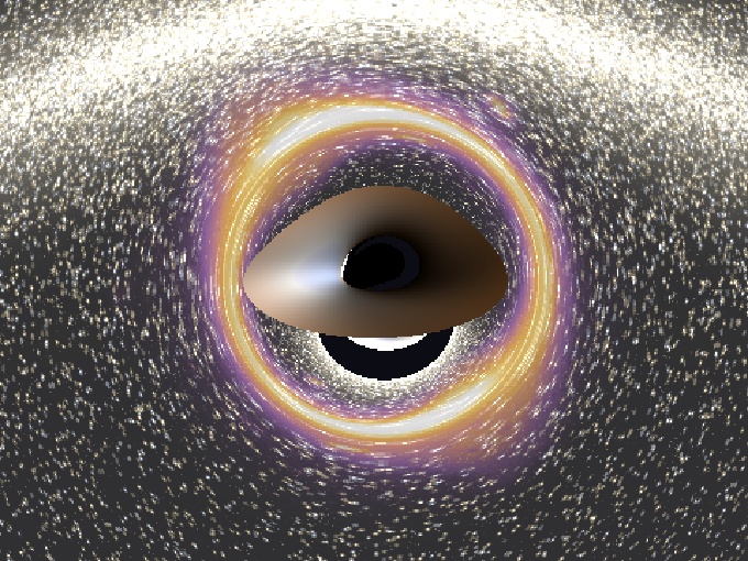
There is already a healthy stack of black-hole posts on Wolfram Community (see the References section). Specifically, what this notebook contributes on top of that prior work is:
◼
an end-to-end reproducible WL build pipeline -- a small package plus three .wls scripts (sky panorama, gallery renders, notebook assembly) that re-run from a single command, rather than a single monolithic notebook;
◼
a Novikov-Thorne thin-disk emission model with Planck-blackbody colour and relativistic beaming I ~ g^4, replacing the hand-rolled colormap that the related posts use;
◼
a composited 'real sky' panorama -- procedural Milky Way starfield plus M31 Andromeda placed within a few degrees of the camera antipode -- so the gravitationally lensed galaxy behind the black hole renders as a recognisable galaxy arc, not just a brighter ring;
◼
a live demonstration that RemoteBatchSubmit on the default WolframBatch environment renders each Kerr frame as one cloud job in roughly the wall-time of a single frame, with explicit cost numbers attached (Section 10).
2. The Kerr metric
2. The Kerr metric
In Boyer-Lindquist coordinates the Kerr line element depends on the two parameters (mass) and (angular momentum per unit mass). We work in geometric units, , so and are measured in units of . Two auxiliary quantities appear everywhere:
{t,r,θ,ϕ}
M
a
Gc1
r
λ
M
Σ+(θ)
2
r
2
a
2
cos
Δ-2Mr+
2
r
2
a
The outer event horizon is the largest root of :
Δ0
r
+
2
M
2
a
The static limit (the outer surface of the ergosphere) is
r
erg
2
M
2
a
2
cos
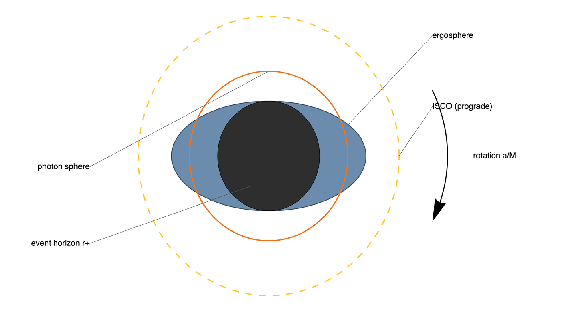
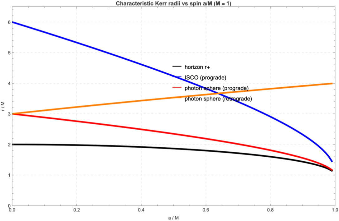
Two more characteristic radii matter for what we are about to render. The first is the circular photon orbit -- the unstable null circular geodesic at radius where a photon can in principle orbit the black hole indefinitely. In Kerr there are two of them (one for prograde, one for retrograde motion):
r
ph
+
r
ph
2
3
-1
cos
a
M
-
r
ph
2
3
-1
cos
a
M
The second is the innermost stable circular orbit -- the inner edge of any geometrically thin accretion disk in the equatorial plane. Bardeen, Press and Teukolsky (1972) found the closed form
r
ISCO
Z
1
3
1-
2
a
2
M
3
1+
+a
M
3
1-
a
M
Z
2
3
2
a
2
M
2
Z
1
r
ISCO
Z
2
(3-)(3++2)
Z
1
Z
1
Z
2
with the minus sign for prograde and the plus sign for retrograde orbits. Prograde ISCO collapses from 6 M (Schwarzschild) to M for an extremal Kerr; this is what makes high-spin disks compact and dramatic.
3. Where the Kerr metric comes from
3. Where the Kerr metric comes from
We have so far taken the Kerr metric as given. It is worth recording briefly that this is not an arbitrary ansatz -- it is the unique spacetime geometry satisfying four reasonable physical assumptions:
◼
stationary -- a timelike Killing vector field exists, so the geometry does not change with time;
◼
axisymmetric -- a spacelike Killing vector field with closed orbits exists, so the geometry is symmetric under rotation about a chosen axis;
◼
asymptotically flat -- far from the source the metric tends to Minkowski;
◼
vacuum -- the energy-momentum tensor vanishes, equivalently 0.
R
μν
The most general stationary axisymmetric metric in Weyl-Lewis-Papapetrou coordinates (Lewis 1932, Papapetrou 1953) can be written
2
ds
2
(t-ωϕ)
2
(ρ)
2
(z)
2
ρ
2
(ϕ)
where , and are functions of the cylindrical radius and axial coordinate only. Substituting this into the vacuum field equations 0 yields, after some algebra, that all the constraints collapse into a single complex equation for the Ernst potential (Ernst 1968):
ν
γ
ω
ρ
z
R
μν
ϵexp(2ν)+
ω
Re(ϵ)ΔϵGrad[ϵ].Grad[ϵ]
Carter (1971) and Robinson (1975) proved that the asymptotically flat solutions of this equation that have a regular event horizon form a single two-parameter family, the Kerr family, parametrised exactly by mass and angular momentum . In Boyer-Lindquist coordinates the Kerr line element is
M
JaM
2
ds
2Mr
Σ
2
(t)
(4Mar(θ))tϕ
2
sin
Σ
Σ
2
(r)
Δ
2
(θ)
(-Δ(θ))(θ)
2
(+)
2
r
2
a
2
a
2
sin
2
sin
2
(ϕ)
Σ
with and as defined in Section 2. We can verify directly in Wolfram Language that this metric is indeed a vacuum solution by computing its Ricci tensor from the Christoffel symbols and asking Simplify to reduce each component:
Σ+(θ)
2
r
2
a
2
cos
Δ-2Mr+
2
r
2
a
coords={t,r,θ,ϕ};Σval=r^2+a^2Cos[θ]^2;Δval=r^2-2Mr+a^2;g={{-(1-2Mr/Σval),0,0,-(2MarSin[θ]^2)/Σval},{0,Σval/Δval,0,0},{0,0,Σval,0},{-(2MarSin[θ]^2)/Σval,0,0,((r^2+a^2)^2-Δvala^2Sin[θ]^2)Sin[θ]^2/Σval}};ginv=Simplify@Inverse[g];Γ=Table[Simplify[(1/2)Sum[ginv[[k,l]](D[g[[l,j]],coords[[i]]]+D[g[[l,i]],coords[[j]]]-D[g[[i,j]],coords[[l]]]),{l,4}]],{k,4},{i,4},{j,4}];ricci=Table[Simplify@Sum[D[Γ[[k,j,i]],coords[[k]]]-D[Γ[[k,k,i]],coords[[j]]]+Sum[Γ[[k,k,l]]Γ[[l,j,i]]-Γ[[k,j,l]]Γ[[l,k,i]],{l,4}],{k,4}],{i,4},{j,4}];MatrixForm@Simplify@ricci(*the4x4zeromatrix*)
The full simplification takes a minute or two on a modern laptop, but every component reduces to 0 -- Kerr is genuinely a vacuum solution.
4. Null geodesics and Carter's constant
4. Null geodesics and Carter's constant
The azimuthal motion is given by
5. From image-plane to conserved quantities
5. From image-plane to conserved quantities
6. Wolfram Language implementation
6. Wolfram Language implementation
and the photon redshift factor between an observer at infinity and the disk fluid (the ratio of observed to emitted photon energies) is
Second, the local rest-frame temperature. We use the Shakura-Sunyaev / Novikov-Thorne thin-disk profile:
projected to RGB through a Tanner-Helland colour-temperature approximation (which is fast, branchless and accurate to a few percent across the visible band).
The full implementation lives in the package KerrRayTracerWL.wl. The core entry point is KerrRayTrace -- it loops over pixels, builds the conserved quantities, calls NDSolveValue on Hamilton's equations with three WhenEvent terminators (horizon, disk, escape), and colours the pixel accordingly:
Before running any of the rendering cells below, save the bundled KerrRayTracerWL.wl and background_realistic.png files in the same directory as this notebook, then evaluate the cell below (Cell > Evaluate Initialization Cells):
Two modelling choices are worth flagging:
DiskModel -> "NovikovThorne" replaces the empirical disk colour ramp with a Shakura-Sunyaev / Novikov-Thorne radial temperature profile T_rest(r) = T_in (r_in/r)^{3/4} (1 - sqrt(r_in/r))^{1/4}, an apparent temperature T_obs = g T_rest (combined gravitational redshift and Doppler), RGB colour from the Planck spectrum, bolometric intensity I ~ g^4 from the relativistic Liouville invariant, and a mild log-spiral modulation. The inner-edge blueshifted side comes out as a near-white hot spot, the outer / receding side as deep orange-red. "Empirical" recovers the v1 hand-rolled colour ramp for backwards compatibility.
BackgroundImage -> bgRealistic is the composited sky built by build_realistic_sky.wls: a procedural Milky Way starfield with a galactic plane and central bulge, M31 Andromeda placed at galactic coordinates (l, b) = (Pi, -0.35 rad), and M42 Orion placed off-axis. The (Pi, -0.35) position sits within about 3 degrees of the antipode of the default observer colatitude theta_0 = Pi/2 - 0.4, close enough that the rays which skim the photon sphere sample directly through M31 and form a visibly lensed arc around the shadow.
7. Spin gallery
7. Spin gallery
As we increase the dimensionless spin a/M from 0 (Schwarzschild) up to the Thorne bound 0.998, two things happen: (i) the photon ring narrows and grows asymmetric -- the prograde side comes in closer to the horizon, the retrograde side pulls outward; (ii) the inner disk eats further inward because the ISCO collapses toward r = M for prograde orbits.
8. Edge-on view: the photon-sphere knife edge
8. Edge-on view: the photon-sphere knife edge
Looking almost edge-on at the disk reveals the dramatic warping predicted by Luminet (1979) and made famous by Interstellar (Thorne 2014). The far side of the disk is bent up over the top of the black hole, and a second, brighter ring -- the photon ring -- traces the photon sphere itself.
9. Where the background comes from
9. Where the background comes from
The celestial sphere texture is built by the bundled build_realistic_sky.wls script. It composites three layers: (i) a procedural Milky Way starfield -- ~220 k stars drawn from a power-law luminosity function and three stellar colour families (G-K-M, A-F, O-B) at the canonical 60 / 30 / 10 percent weights, with a galactic-plane density concentration and a Gaussian central bulge; (ii) the M31 Andromeda image from my AstronomyImages project (DSS / 2MASS through SkyView), soft-edged into the sky at galactic coordinates (l, b) = (Pi, -0.35 rad); (iii) the M42 Orion nebula composited off-axis as a secondary feature.
The (Pi, -0.35 rad) position is not random: it is within about 3 degrees of the antipode of the default observer colatitude theta_0 = Pi/2 - 0.4, close enough that rays which skim the photon sphere sample directly through M31 and produce the visibly lensed Einstein-ring arc right outside the shadow. Photons that escape at wider angles sample the Milky Way plane and halo stars, so the rest of the sky is populated rather than stretched copies of a single galaxy image.
10. Cinematic video via RemoteBatchSubmit
10. Cinematic video via RemoteBatchSubmit
A single Kerr frame takes a minute or two locally; a 60-frame 4K fly-around would take days. Wolfram's RemoteBatchSubmit changes that almost completely: each frame is one self-contained Wolfram expression, so we submit them all in parallel to a cloud batch service and the whole video finishes in roughly the wall time of a single frame.
The pleasant surprise is how little plumbing this needs. Every cloud-connected Wolfram installation already has a working default environment, $DefaultRemoteBatchSubmissionEnvironment, that points at the WolframBatch backend. No AWS account, no IAM policy, no Docker images, no $RemoteBatchSubmissionEnvironment to configure -- you just call RemoteBatchSubmit on the Wolfram expression you want evaluated, and the result comes back as job["EvaluationResult"]. The package wraps this in KerrRayTraceRemote and KerrVideoRemote so a one-frame submission and a sixty-frame video look almost identical.
Here is the single-frame call. Submitted to the default WolframBatch environment, this 120x90 frame runs in roughly a minute of wall time end-to-end:
And the fly-around video. Each of the 60 frames becomes one RemoteBatchSubmit job, all running in parallel; the encoder stitches them into mp4 when every job has reached terminal status:
Internally each frame is submitted as one self-contained RemoteBatchSubmit expression. Because RemoteBatchSubmit has the HoldAll attribute, we can write KerrRayTrace[...] directly without any Hold[...] wrapper, and the IncludeDefinitions -> True default bundles all local definitions automatically -- so the worker simply receives the unevaluated call, evaluates it, and returns an Image which the client picks up via job["EvaluationResult"].
Worked example. Running KerrRayTraceRemote with Provider -> "WolframBatch" on a 120x90 frame returned an Image of the expected dimensions in roughly 70 seconds of total wall time -- about 4 seconds to submit, ~30 seconds in the WolframBatch queue, ~35 seconds running on a Basic1x8 worker. Per-job credit cost was 20 000 credits (about US$0.10 at the standard Wolfram Cloud rate). Switching to a larger machine class (RemoteMachineClass option) brings that down further at proportionally higher cost; submitting an AWS-Batch environment as 'Environment' -> RemoteBatchSubmissionEnvironment["AWS", ...] also works.
Scaling from the empirical Basic1x8 measurement (10 800 rays in 73.8 s wall, 20 000 credits ~ US$0.10):
◼
per-ray cost: ~9.3 x 10^-6 USD per ray
◼
per-ray time: ~6.8 ms per ray on Basic1x8
◼
640 x 480 frame: ~35 min wall, ~$2.85
◼
1080p frame: ~3.9 hr wall, ~$19
◼
4K frame: ~16 hr wall, ~$77
◼
4K 60-frame video, fully parallel (60 jobs in flight): ~16 hr wall, ~$4600 total
These are rough projections under the (linear in pixel count) assumption that the per-ray cost is constant; moving to a larger RemoteMachineClass cuts wall time at proportionally higher cost. A small proof-of-pipeline 240x180 video, rendered serially on a laptop in ~11 minutes, sits at videos/kerr_test_inclination_sweep.mp4 in this repo.
And as a quick local smoke test, with Provider -> "Local" the same function dispatches the per-tile renderTile calls through ParallelMap on local kernels:
With Provider -> "Local" the call tiles the image and dispatches the per-tile renders through ParallelMap on local kernels. With Provider -> "WolframBatch" (the package default) the entire frame is submitted as one self-contained RemoteBatchSubmit job to the cloud worker; the worker evaluates KerrRayTrace[...] with the bundled definitions and returns an Image which the local kernel picks up via job["EvaluationResult"]. The practical appeal is that you write Wolfram code, you test it locally, and the only line that changes between a 1-minute laptop render and a 4K 60-frame video on the cloud is the value of one option.
11. A cinematic alternative: a 360-degree GPT-image-2 panorama
11. A cinematic alternative: a 360-degree GPT-image-2 panorama
Everything above is a physically motivated ray trace in pure Wolfram Language. As a complement -- and a useful reminder of where AI image generation currently sits -- it is also possible to ask GPT-image-2 to draw a black hole directly, with no underlying GR computation, and then drop the result into a Wolfram viewer. The image is striking but is artwork, not physics. It does, however, make a very effective hook.
The single prompt used was, verbatim:
"Could you make a 360 degree image of the view of a Kerr black hole? Behind it there should be the galaxy and we should be able to look all around. There needs to be a high resolution. Think through how the light would bend and what exactly I would see. Make the accretion disk realistic."
The model returned a 1774 x 887 equirectangular panorama (suitable to texture onto a sphere):
The Wolfram-side viewer fits in a few lines: load the 2:1 equirectangular image, texture it onto the inside of a unit sphere with SphericalPlot3D, and wrap the result in a Manipulate with yaw and pitch sliders. The full file (with the panorama itself embedded as a base64 string so it is self-contained) is bundled alongside this notebook as blackhole_viewer.wl; the entry-point call is just
For a quick web-native version, a hosted drag-to-pan instance lives at claude.ai/public/artifacts/1844fad3.... A self-contained blackhole_viewer.html is also bundled alongside this notebook -- save it next to kerr.nb and open it in any modern browser. Drag, scroll to zoom, and watch the lensed disk drift across the field of view. None of it is GR-correct -- but together with the physics-based renders above, it makes the contrast between an LLM's intuition about a black hole and the actual general-relativistic geometry very explicit.
12. Acknowledgements for external material
12. Acknowledgements for external material
Astronomical sky imagery. The M31 Andromeda and M42 Orion frames composited into the equirectangular sky panorama come from the sister repository AstronomyImages, which pulls Digitized Sky Survey (DSS) and 2MASS plate data through NASA's SkyView Virtual Observatory. The standard required acknowledgement follows: "The Digitized Sky Surveys were produced at the Space Telescope Science Institute under U.S. Government grant NAG W-2166. This work makes use of data products from the Two Micron All Sky Survey, a joint project of the University of Massachusetts and the Infrared Processing and Analysis Center / California Institute of Technology, funded by NASA and NSF. This research has made use of NASA's SkyView facility (https://skyview.gsfc.nasa.gov) located at NASA Goddard Space Flight Center."
AI-generated images. Three of the four section-header infographics (geodesics, Doppler, ray-tracing pipeline) and the 360-degree black-hole panorama used in Section 11 were generated by OpenAI's gpt-image-2 image model. Image outputs of gpt-image-2 are made available to the prompting user under OpenAI's content policy.
13. References
13. References
Primary literature:
Primary literature:
◼
Kerr, R. P. (1963). Gravitational Field of a Spinning Mass.
◼
Carter, B. (1968). Global structure of the Kerr family.
◼
Bardeen, Press, Teukolsky (1972). Rotating black holes.
◼
Bardeen, J. M. (1973). Timelike and null geodesics in Kerr.
◼
Novikov, I. D. and Thorne, K. S. (1973). Astrophysics of black holes (in Black Holes / Les Astres Occlus).
◼
Luminet, J.-P. (1979). Image of a spherical black hole with thin disk.
◼
Thorne et al. (2015). Gravitational lensing by spinning black holes (Interstellar).
◼
Event Horizon Telescope Collaboration (2019, 2022). First M87 and SgrA results.
Related Wolfram Community posts on black-hole visualisation:
Related Wolfram Community posts on black-hole visualisation:
◼
Jingxian Wang, How black holes and accretion disks around them actually look, Wolfram Community (2020). The closest analogue to this post -- a full Schwarzschild render of an accretion disk including Doppler, gravitational lensing and light-travel time effects, comparing the result to the Interstellar visualisation.
◼
Lihang Zhou, Forward ray tracing and hot spots in Kerr spacetime, Wolfram Community (2025). A complementary forward-tracing approach (emission point -> observer) applied to time-variable hot spots in the Kerr disk -- useful for connecting our backward-trace renders to the EHT observational picture.
◼
Alex Lupsasca, Black Hole Vision: an interactive iOS application for visualizing black holes, Wolfram Community (2026). Real-time mobile renderer from one of the EHT theorists; aimed at intuition rather than physical fidelity, but a useful companion for playing with viewpoints.
◼
Michael Ostroff, Geodesics around a Kerr black hole, Wolfram Community (2023). Detailed treatment of the Carter-separated geodesic equations and their numerical integration -- the same physics the KerrRayTracerWL package uses for each pixel ray.
◼
Pablo A. Cano, Rotating black holes: corrections to the Kerr metric package, Wolfram Community (2020). Higher-derivative gravity corrections to the Kerr metric; companion to Cano-Fransen-Hertog (Phys. Rev. D 102, 044047, 2020).
◼
Additional related threads: The Kerr-Newman black hole, Kerr geodesics in terms of Weierstrass elliptic functions, and the WSC/WSS notebooks Visualizing a Binary Black Hole Merger and Hunting for black holes.
CITE THIS NOTEBOOK
CITE THIS NOTEBOOK
Painting a Kerr black hole: a backward null-geodesic ray tracer with a real astrophotograph
by Marco Thiel
Wolfram Community, STAFF PICKS, May 15, 2026
https://community.wolfram.com/groups/-/m/t/3716438
by Marco Thiel
Wolfram Community, STAFF PICKS, May 15, 2026
https://community.wolfram.com/groups/-/m/t/3716438