Problem
Problem
Calculate the first 10 terms of the Taylor series for the function . In a common graph, plot the above Taylor polynomial of the function along with the function itself in the interval
f(x)exp(-0.1x)sin(x)
f(x)
f(x)
x∈[0,2π]
The first 10 terms of the Taylor series for the function are :
f(x)exp(-0.1x)sin(x)
x-0.1-0.16166666666666665+0.0165+0.007504166666666667-0.0008056388888888889-0.0001574390873015873+0.00001846625+1.7981594190917109-2.4319554949294534
2
x
3
x
4
x
5
x
6
x
7
x
8
x
-6
10
9
x
-7
10
10
x
In[]:=
f[x_]:=Exp[-0.1*x]*Sin[x];taylor=Normal[Series[f[x],{x,0,10}]];taylor
Out[]=
x-0.1-0.161667+0.0165+0.00750417-0.000805639-0.000157439+0.0000184663+1.79816×-2.43196×
2
x
3
x
4
x
5
x
6
x
7
x
8
x
-6
10
9
x
-7
10
10
x
In[]:=
Plot[{f[x],taylor},{x,0,2Pi},PlotLegends->{"f(x)","Taylor Series"}]
Out[]=
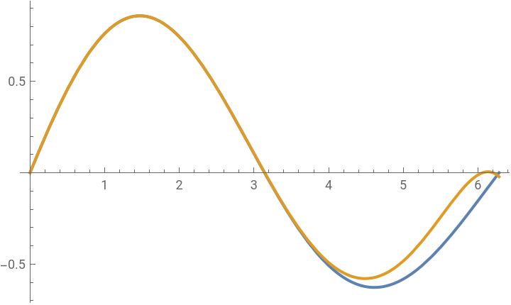


The Taylor series is a way to represent a function as an infinite sum of terms that are calculated from the values of the function' s derivatives at a single point . In this case, we have calculated the first 10 terms of the Taylor series for the function around the point . The resulting polynomial is : This polynomial is an approximation of the original function near . The more terms we include in the series, the better the approximation will be, and the larger the interval around within which the approximation is good . However, it' s important to note that the Taylor series does not always converge to the function it' s approximating, especially for values of far from the point around which the series is calculated (in this case, ) . This is evident from the plot we generated earlier, where the Taylor approximation starts to diverge from the original function as moves away from 0.In conclusion, the Taylor series provides a powerful tool for approximating functions with polynomials, especially near a specific point . But care must be taken when using these approximations, as they may not be accurate over large intervals or for complex functions .
f(x)exp(-0.1x)sin(x)
x0
x-0.1-0.16166666666666665+0.0165+0.007504166666666667-0.0008056388888888889-0.0001574390873015873+0.00001846625+1.7981594190917109-2.4319554949294534
2
x
3
x
4
x
5
x
6
x
7
x
8
x
-6
10
9
x
-7
10
10
x
f(x)
x0
x0
x
x0
x
We will do the same for Fourier Series and then we will compare the two cases.
We will do the same for Fourier Series and then we will compare the two cases.
The first 10 terms of the Fourier series for the function are :
f(x)exp(-0.1x)sin(x)
-0.10064660454698496+(0.025349892915823936+0.5069978583164828i)+(0.025349892915823936-0.5069978583164828i)+(0.033399927591063826-0.004468217737934933i)+(0.033399927591063826+0.004468217737934933i)-(0.012651195777478754-0.0009500272173325569i)-(0.012651195777478754+0.0009500272173325569i)+(0.006762132120208066-0.0003608876381698658i)+(0.006762132120208066+0.0003608876381698658i)-(0.004229960349193359-0.00017632181530609237i)-(0.004229960349193359+0.00017632181530609237i)+(0.0029017904693091085-0.00009951839277424079i)+(0.0029017904693091085+0.00009951839277424079i)-(0.00211641242780506-0.00006174155863569073i)-(0.00211641242780506+0.00006174155863569073i)+(0.0016127564051439662-0.00004096539527274201i)+(0.0016127564051439662+0.00004096539527274201i)-(0.0012701790462557336-0.000028582601365920143i)-(0.0012701790462557336+0.000028582601365920143i)+(0.0010264834056544576-0.00002073913336002128i)+(0.0010264834056544576+0.00002073913336002128i)
ix
e
-ix
e
2ix
e
-2ix
e
3ix
e
-3ix
e
4ix
e
-4ix
e
5ix
e
-5ix
e
6ix
e
-6ix
e
7ix
e
-7ix
e
8ix
e
-8ix
e
9ix
e
-9ix
e
10ix
e
-10ix
e
In[]:=
f[x_]:=Exp[-0.1*x]*Sin[x];fourier=FourierSeries[f[x],x,10];fourier
Out[]=
-0.100647+(0.0253499+0.506998)+(0.0253499-0.506998)+(0.0333999-0.00446822)+(0.0333999+0.00446822)-(0.0126512-0.000950027)-(0.0126512+0.000950027)+(0.00676213-0.000360888)+(0.00676213+0.000360888)-(0.00422996-0.000176322)-(0.00422996+0.000176322)+(0.00290179-0.0000995184)+(0.00290179+0.0000995184)-(0.00211641-0.0000617416)-(0.00211641+0.0000617416)+(0.00161276-0.0000409654)+(0.00161276+0.0000409654)-(0.00127018-0.0000285826)-(0.00127018+0.0000285826)+(0.00102648-0.0000207391)+(0.00102648+0.0000207391)
-x
x
-2x
2x
-3x
3x
-4x
4x
-5x
5x
-6x
6x
-7x
7x
-8x
8x
-9x
9x
-10x
10x
The Fourier series is a way to represent a periodic function as a sum of sine and cosine functions . It' s especially useful for analyzing and manipulating functions that are periodic . In this case, the Fourier series provides a representation of the function in terms of complex exponentials, which are equivalent to sines and cosines .
(f(x)
In[]:=
Plot[{f[x],fourier},{x,0,2Pi},PlotLegends->{"f(x)","Fourier Series"}]
Out[]=
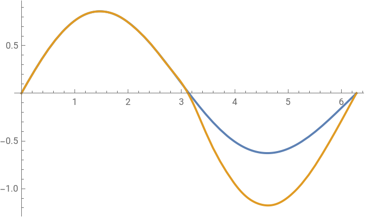
In this case, we have computed the first 10 terms of the Fourier series for the function . The result is a complex series, which can be interpreted as a sum of sine and cosine functions with different amplitudes and phases . Each term in the series corresponds to a specific frequency, and the coefficient of each term indicates the strength (or amplitude) and phase shift of that frequency component in the original function . It' s important to note that the Fourier series provides an exact representation of the function only if the function is periodic and satisfies certain mathematical conditions (like being piecewise smooth) . For other functions, the Fourier series provides an approximation . The more terms we include in the series, the better the approximation . In this specific case, the function is not strictly periodic, so the Fourier series provides an approximation . The quality of the approximation would depend on the specific range of values we' re interested in . Finally, the Fourier series is a powerful tool in mathematics and engineering, but interpreting its results can require a good understanding of concepts like frequency, amplitude, phase, and complex numbers .
f(x)exp(-0.1x)sin(x)
f(x)exp(-0.1x)sin(x)
x
Conlusion
Conlusion
We have the function , which is a product of an exponential function and a sine function . This function is not strictly periodic, but it does have a periodic component due to the term . The Taylor series expansion of this function provides a polynomial approximation that is particularly accurate near the point of expansion, which in our case was . As we move away from this point, the Taylor approximation becomes less accurate . This is a general property of Taylor series : they provide local approximations that are accurate within a certain radius of the point of expansion . On the other hand, the Fourier series expansion provides a representation of the function in terms of sine and cosine functions (or complex exponentials) . This captures the periodic nature of the part of the function, but it' s important to note that the Fourier series is an infinite series, and we' ve only computed the first 10 terms . Therefore, the Fourier series we' ve computed is an approximation of the function, and its accuracy would improve as more terms are included . In comparing the two, the Taylor series gives a good approximation near , while the Fourier series captures the oscillatory behavior of the function . The choice between using a Taylor series or a Fourier series would depend on what aspects of the function you' re most interested in (e . g ., behavior near a specific point versus periodic behavior), and what you know about the function (e . g ., whether it' s periodic) .
f(x)exp(-0.1x)sin(x)
sin(x)
x0
sin(x)
x0