Watching an earthquake cross a continent: vertical ground motion at the European seismic network as the 2025 Myanmar M7.7 wavefronts arrive (red = up, blue = down). Built from scratch below — see §7.
When the ground breaks, it rings the whole planet like a bell. Within 20 minutes the wavefronts of a great earthquake have swept past every seismometer on Earth, and the precise pattern of their arrival encodes the interior structure of our planet – and the nature of the source that set them off. This notebook builds that physics from first principles in pure Wolfram Language: the elastic wave equation, the PREM velocity model, ray theory in a spherical Earth, and the travel-time integrals that we validate against the IASP91 standard to within a few seconds. We then turn the same machinery on a question of real consequence – how seismology tells an underground nuclear explosion apart from an earthquake.
Setup
Setup
This post is fully runnable. All of the computational machinery – the PREM model, the ray tracer, the travel-time integrals, the event catalogue, the energy and discrimination tools and the Ground Motion Visualization engine – lives in the companion package SeismicWavePropagation.wl, which sits in the same folder as this notebook. Evaluate the cell below first to load it (it computes the P and S travel-time curves on load, so it takes roughly half a minute). Every figure that follows is produced by the call shown directly above it. Note: the map and globe figures use GeoGraphics with a relief background, which needs an internet connection; the real-data figures (§11, §7) read the committed CSVs in data/ and run offline.
SetDirectory[NotebookDirectory[]];Get["SeismicWavePropagation.wl"]
1 | What is an earthquake?
1 | What is an earthquake?
The outer shell of the Earth is broken into rigid plates that grind past one another. Friction locks their boundaries, elastic strain accumulates in the surrounding rock for decades or centuries, and when the stress finally exceeds the strength of the fault the two sides snap past each other in seconds. This is elastic rebound: the stored strain energy is released, and a fraction of it radiates away as seismic waves.
Those waves come in two families. Body waves travel through the Earth's interior – the compressional P-wave (fastest, arrives first) and the shear S-wave. Surface waves (Rayleigh and Love) are trapped near the free surface, travel more slowly, but carry the largest amplitudes and do most of the damage. The rest of this notebook is, in essence, a careful account of how fast each of these travels and why.
2 | The physics of seismic waves
2 | The physics of seismic waves
Small deformations of an isotropic elastic solid obey the elastic wave equation. It separates into two independent solutions. The compressional and shear wave speeds are set entirely by the elastic moduli (Lamé parameter λ, shear modulus μ) and the density ρ:
v
P
λ+2μ
ρ
v
S
μ
ρ
Two physical facts fall straight out of these formulas. First, because λ and μ are positive, > always – the P-wave outruns the S-wave, which is why P stands for primary and S for secondary. Second, a fluid cannot support shear (μ = 0), so = 0 there: S-waves do not propagate through liquids. That single fact is how we know the outer core is molten. For a typical Poisson solid the ratio is fixed:
v
P
v
S
v
S
v
P
v
S
3
≈1.733 | The PREM velocity model
3 | The PREM velocity model
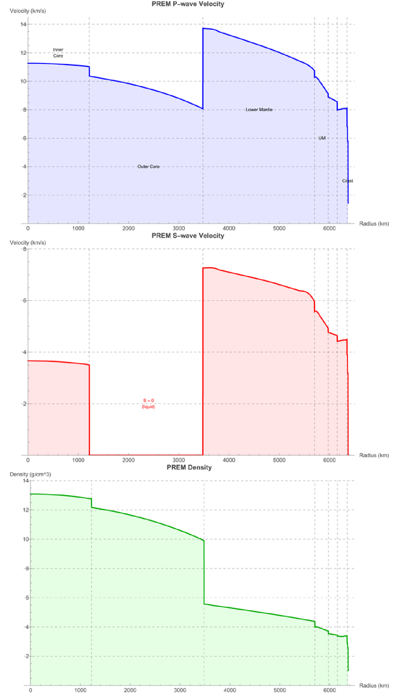
To trace waves through the Earth we need the seismic velocity at every depth. We use the Preliminary Reference Earth Model (PREM, Dziewonski & Anderson 1981), the standard spherically averaged model. Tabulated node-by-node and interpolated layer by layer, it captures the major internal boundaries: the inner-core boundary at 1221.5 km radius, the core–mantle boundary (CMB) at 3480 km, and the 660 km and 410 km mantle phase transitions.
plotPREMProfiles[]
PREM P-wave and S-wave velocity and density as a function of radius. Note vS = 0 throughout the liquid outer core. |
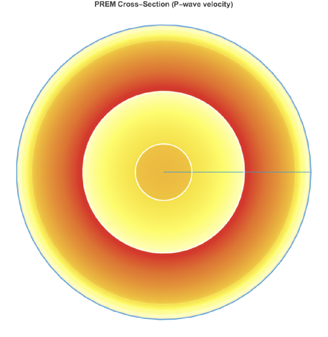
Mapping the P-wave velocity onto a cross-section shows the same structure as concentric shells – velocity generally increasing with depth, with sharp jumps at the boundaries:
plotPREMCrossSection[]
PREM P-wave velocity as a cross-section of the Earth (warmer = faster). |
4 | Ray theory and travel times
4 | Ray theory and travel times
In a spherically symmetric Earth, a seismic ray obeys Snell's law in spherical coordinates. The combination
p==const
rsini
v(r)
is conserved along the entire path – this is the ray parameter. Introducing the radial slowness , a ray turns horizontal () at the radius where . The epicentral distance and travel time follow as integrals over the up-going path:
η(r)=r/v(r)
i=90°
r
tp
η()=p
r
tp
Δ(p)=2r
R
∫
r
tp
p
r-
2
η
2
p
T(p)=2r
R
∫
r
tp
2
η
r-
2
η
2
p
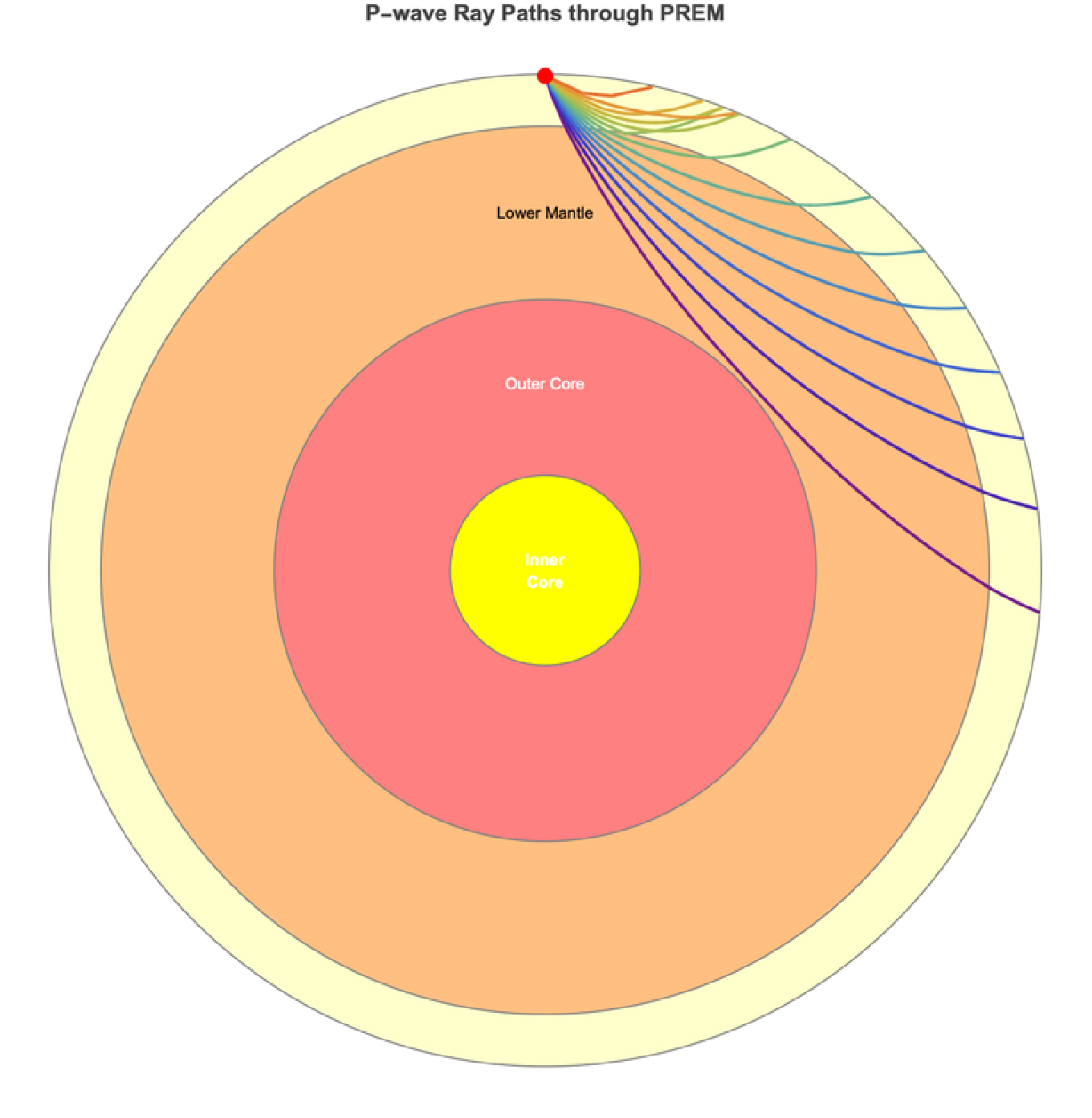
These integrals have an integrable singularity at the turning point, where the square root vanishes. We tame it with the substitution , which makes the integrand regular and gives accurate, real-valued results. Sweeping p from the core–mantle boundary up to the surface traces every ray of the direct branch:
r=+
r
tp
2
ξ
plotRayPaths[]
P-wave ray paths through PREM. Shallow rays (red) emerge close by; deeper-turning rays (blue–purple) bottom near the core–mantle boundary and emerge near 95°. (Rays are drawn from the source at the Moho; the thin crustal leg is omitted for clarity.) |
How good is this from-scratch calculation? Comparing the computed P times against the IASP91 standard reference (Kennett & Engdahl 1991) shows agreement to within a few seconds across teleseismic distances – the verification table is in §11.
5 | Seismic energy and magnitude
5 | Seismic energy and magnitude
The numbers are sobering: the 1960 Chile M9.5 released on the order of 10,000 times the energy of the 250 kt DPRK test; even the Tohoku M9.1 released roughly 2,700 times as much.
6 | A global tour of recent events
6 | A global tour of recent events
We anchor the physics in seven real events – six earthquakes spanning four orders of magnitude in energy, plus one underground nuclear test:
7 | Watching the waves sweep the planet
7 | Watching the waves sweep the planet
This is where the physics becomes visible. A Ground Motion Visualization (GMV), pioneered by IRIS, animates the vertical ground motion recorded at many seismometers: each station is a dot that turns red when the ground heaves up and blue when it drops. Here is the real Mandalay M7.7 – actual LHZ waveforms from 73 European stations (FDSN / IRIS-EarthScope), band-passed and normalised. Watch the wave sweep in from the east: the stations nearest the source (the Caucasus) light up first and hardest, then the disturbance rolls across the continent to Iberia:
Now compare that with the synthetic GMV at the top of this post. That one uses no data at all – a 2000-station synthetic network and seismograms generated purely from the PREM travel-time model above – yet it reproduces the same eastward sweep. The physics alone predicts what the real network records. (Its full-resolution 25-second video is docs/images/SeismicGMV.mp4; the synthetic engine is exportGMVFrames[event].)
The same event as idealized wavefronts
The same event as idealized wavefronts
8 | Supershear rupture
8 | Supershear rupture
9 | Nuclear explosions as seismic sources
9 | Nuclear explosions as seismic sources
An underground nuclear explosion is also a seismic source – but a fundamentally different one. An earthquake is a double-couple: slip on a fault, which radiates both P and S waves with a four-lobed pattern. An explosion is, to first order, isotropic: it pushes outward equally in all directions, radiating an efficient P-wave and almost no shear or surface waves.
Body-wave magnitude scales with yield through an empirical calibration (Murphy 1996):
10 | Telling bombs from earthquakes
10 | Telling bombs from earthquakes
The source physics is even clearer when watched directly. Place a hypothetical double-couple earthquake and the real isotropic explosion at the same spot and let the wavefronts run: the earthquake sprouts an S-front and a Rayleigh front; the explosion shows only the P-front. That missing shear energy is the signature of an explosion:
The radiation patterns make the same point statically – the four-lobed double-couple beside the uniform explosion:
11 | Verifying the model
11 | Verifying the model
The real test: a real earthquake
The real test: a real earthquake
Tables are one thing; the actual Earth is another. So we fetch real broadband seismograms of the Mandalay M7.7 from the global seismic network (FDSN / IRIS-EarthScope), band-pass them to 0.02–0.1 Hz, and lay them out as a record section – amplitude vs. time, each trace offset by its epicentral distance. Onto that we draw the P, S and Rayleigh curves from our PREM model above (a smooth fit through the computed direct-branch times). If the physics is right, the predicted curves should fall on the real arrivals:
The agreement is immediate: the large surface waves ride the orange Rayleigh line at every distance, and the first energy arrives on the blue P curve. Zooming in on a single station – Obninsk, Russia, at 55° – shows all three components (the horizontal channels are LHZ's companions LH1/LH2, oriented ≈ N/E), with the arrivals marked at our predicted times. Note the S wave is stronger on the horizontals than on the vertical, exactly as shear-wave physics demands:
12 | Conclusions
12 | Conclusions
Starting from the elastic wave equation and one tabulated velocity model, we reconstructed the seismologist's toolkit: P and S body waves, the PREM Earth, ray-traced travel times validated against the international standard, the energy–magnitude scaling, global wavefront animations, supershear Mach cones, and the source physics that lets a seismic network distinguish a bomb from a quake. The same handful of equations carries us from why the S-wave is slower all the way to how we verify a nuclear test ban.
Everything here is reproducible pure Wolfram Language – see the note below.
References
References
[1] Dziewonski, A. M. & Anderson, D. L. (1981). Preliminary Reference Earth Model. Phys. Earth Planet. Inter. 25, 297–356.
[2] Shearer, P. M. (2009). Introduction to Seismology. Cambridge University Press.
[3] Kennett, B. L. N. & Engdahl, E. R. (1991). Traveltimes for global earthquake location and phase identification (IASP91). Geophys. J. Int. 105, 429–465.
[4] Kanamori, H. (1977). The energy release in great earthquakes. J. Geophys. Res. 82, 2981–2987.
[5] Murphy, J. R. (1996). Types of seismic events and their source descriptions. In Monitoring a CTBT, NATO ASI Series.
[6] CTBTO – Seismic monitoring: https://www.ctbto.org/our-work/monitoring-technologies/seismic-monitoring
Data and imagery credits
Data and imagery credits
Seismograms (§11 record section and single-station trace, and the real-data GMV) were obtained from the FDSN / IRIS-EarthScope irisws-timeseries service – networks GE (GEOFON), II (GSN/IDA), IU (GSN), MN (MedNet), CH, SL and others. Earthquake source parameters are from the USGS and GCMT catalogues (event us7000pn9s). Base maps are rendered with Wolfram Language GeoGraphics (relief and country-border styling). The synthetic GMV uses no real data – its station network and seismograms are generated from the PREM travel-time model above.
Reproducibility
Reproducibility
The entire pipeline is pure Wolfram Language in the companion repository:
◼
community/SeismicWavePropagation.wl – the function library (PREM, ray tracing, travel-time integrals, event catalogue, energy and discrimination, wavefront engine).
◼
wolfram/generate_figures.wls – renders every figure and the two animations into docs/images/ (the GeoGraphics figures need internet for the relief-map tiles).
◼
community/build_notebook.wls – assembles this notebook from the prose and the rendered figures.
◼
tests/verify.wls – checks the P/S travel times against IASP91, the energy ratios, the mb–yield calibration and the supershear angle.
Build it with:
wolframscript -file wolfram/generate_figures.wls
wolframscript -file community/build_notebook.wls
wolframscript -file community/build_notebook.wls
CITE THIS NOTEBOOK
CITE THIS NOTEBOOK
Seismic wave propagation across the globe: earthquakes vs. nuclear explosions
by Marco Thiel
Wolfram Community, STAFF PICKS, July 1, 2026
https://community.wolfram.com/groups/-/m/t/3742365
by Marco Thiel
Wolfram Community, STAFF PICKS, July 1, 2026
https://community.wolfram.com/groups/-/m/t/3742365