Wolfram Cloud Document

ABSTRACT (original article): The manner in which healthy humans interact with objects as they move them within the hand is essential for activities of everyday life. The present study aims to identify the most salient features of the complex interactions between the fingers of the hand and the object. Specifically, the study seeks to determine whether the force applied by a healthy person follows a natural trend throughout the movement, or if it varies from individual to individual. Results will potentially inform the design of therapies, surgeries, and the design of prosthetic and orthotic devices to restore function in patients with compromised hand function. CITATION (original article): Das, D., Schultz, J. Principal Component Analysis of Grasp Force and Pose During In-Hand Manipulation. J. Med. Biol. Eng. 42, 658–670 (2022). https://doi.org/10.1007/s40846-022-00748-x

Methods

The joint angles of four healthy subjects were recorded by a magnetic motion tracking system along with the forces the hand was applying to an instrumented object. These were recorded as subjects moved the object from a pose with fingers outstretched toward the palm of the hand and back again. After the joint angles were extracted from the motion capture readings, principal component analysis was conducted on the joint angle-force space as well as the space consisting of the joint angles alone.

Results

Principal component analysis of the joint angle and force data revealed that the first two principal components explained over 90% of the variance. One of these principal components was associated with the curling motion of the fingers, and the other with the squeezing of the object. The curling motion was consistent from subject to subject, but the changes in gripping force over the course of the movement varied from individual to individual.

Conclusion

The study supports the notion that when conducting an in-hand manipulation of an object, the coupled motions of the fingers and the sequence of hand shapes follows a common trend across individuals. The force applied to the object, however, seems to be volitional on the part of the subject and does not seem to follow as a consequence of the hand movement.

Code

Set file path for Dip’ s Excel file

pcaDirectory="C:\\Users\\jas019\\OneDrive - University of Tulsa\\TUHand\\TUHandshare\\Dip Research";

Needs["PlotLegends`"]

Set the directory to be the file path with Dip’ s Excel file data

SetDirectory[pcaDirectory]

C:\Users\jas019\OneDrive - University of Tulsa\TUHand\TUHandshare\Dip Research

Check to make sure SetDirectory worked

Directory[]

C:\Users\jas019\OneDrive - University of Tulsa\TUHand\TUHandshare\Dip Research

Store the info in the Excel file as a Mathematica List of Lists . The first subscript is the sheet (1-- 4) . Each of the 4 contains a matrix

pcaData=Import["pca.XLSX"];

Count number of sheets in Excel workbook

nosheets=Dimensions[pcaData][[1]];

Generate a list of integers up to nosheets

itertable=Table[i,{i,nosheets}];

Drop the last three rows for each subject, which correspond to forces

pcaAngleData=Map[Drop[#,-3]&,pcaData];

Drop the first four rows for each subject, which correspond to angles

pcaForceData=Map[Drop[#,4]&,pcaData];

Plot[{ArcSin[x],x},{x,0,2},PlotRangeAll]

angledataplots=Map[ListLinePlot[#,PlotStyle{{Blue,Dashed},{Magenta,Dashed},{Green,Dashed},{Cyan,Dashed}}]&,pcaAngleData];

Map[Max[#]&,pcaAngleData]

{0.996298,0.565076,0.681306,0.835141}

Map[Min[#]&,pcaAngleData]

{-0.964891,-0.931057,-0.979004,-0.992289}

Take the arcsin of the angle data, per Dip’ s email July 5

pcaAngleValues=Map[ArcSin[#]&,pcaAngleData];

pcavalueplots=Map[ListLinePlot[#]&,pcaAngleValues];

Check to see the results of the ArcSin function on the data

Show[angledataplots[[1]],pcavalueplots[[1]],PlotRangeAll]

Trim out the start before the first subject starts moving

pcaAngleValues1trim=pcaAngleValues[[1]][[All,11;;-1]];

Sampling rate with downsampling

sampletime=1/(240/16);

maxtime=sampletime*Dimensions[pcaAngleValues1trim][[2]]

107

Generate a list of time values at the downsampled sample instants shown for plotting

timevals=Drop[Table[i,{i,0,maxtime,sampletime}],-1];

Dimensions[timevals]

{107}

Dimensions[pcaAngleValues1trim[[1]]]

{107}

Store time, angle value as ordered pairs for each subject

pcaAngleValues1trimaug=Map[Transpose[{timevals,#}]&,pcaAngleValues1trim];

subj1timedomain=ListLinePlot[pcaAngleValues1trimaug,PlotRange{{0,7},{-1.5,1.5}},PlotStyle{{Blue,Dashed},{Thickness0.008,Magenta,DotDashed,Dashing[{0.01,0.01,0.04,0.01}]},{RGBColor[{0,0.76,0}]},{Thickness0.006,Red,Dotted,Dashing[0.005]}},PlotTheme"Detailed",FrameLabel{"Time [s]","Joint Angle [radians]"},PlotLegends{"MCP flex/ext","MCP abd/add","PIP","DIP"},LabelStyleDirective[FontSize->8],AspectRatio9/16,ImageSize72×3]

	MCP flex/ext
	MCP abd/add
	PIP
	DIP

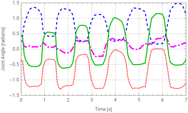
Export["firstsubject.eps",subj1timedomain]

firstsubject.eps

Trim out the start before the first subject starts moving

pcaForceData1trim=pcaForceData[[1]][[All,11;;-1]];

Store time, angle value as ordered pairs for each subject

pcaForceData1trimaug=Map[Transpose[{timevals,#}]&,pcaForceData1trim];

subj1timedomainforce=ListLinePlot[pcaForceData1trimaug,PlotRange{{0,7},{-15,5}},PlotStyle{{Brown,Dashed,Dashing[{0.03,0.01}]},{Thickness0.01,Black,DotDashed,Dashing[{0.01,0.01,0.06,0.01}]},{RGBColor[{0.66,0.66,0}]}},PlotTheme"Detailed",FrameLabel{"Time [s]","Force [N]"},PlotLegends{"x dir","y dir","z dir"},LabelStyleDirective[FontSize->8],AspectRatio9/16,ImageSize72×3]

	x dir
	y dir
	z dir

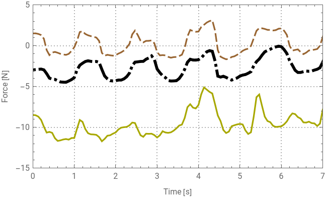
Export["firstsubjectforce.eps",subj1timedomainforce]

firstsubjectforce.eps

Replace the raw angle values in the file with the arcsine of those values, so the value is in radians

pcaDataProc=Map[Join[pcaAngleValues[[#]],pcaForceData[[#]]]&,itertable];

Take the mean of each variable waveform

themeanvals=Map[Mean[#]&,pcaDataProc,{2}]

{{0.798424,0.133433,0.0857857,-0.733666,0.345812,-2.77542,-9.49219},{-0.502645,-0.296273,0.0483642,-0.681338,1.91228,0.651408,-0.305293},{-0.525269,-0.0635647,0.149919,-0.549201,2.55628,-0.553908,-5.13448},{-0.333764,-0.0279523,0.211114,0.540376,0.504539,-0.480183,-1.61489}}

Compute the maximum “squeezing” force for each subject

Transpose the rows and columns of pcaDataProc for each subject to subtract off the mean

Generate a function that subtracts off the mean from an entire list

This generates the data with the mean removed

Extract the mean of the z force

Function that divides columns 5, 6, and 7 of a subject’ s data (the forces) by the max force in the z direction times 2 radians (roughly the range of motion of the mcp flexion)

Normalize the forces so that they have an equivalent range to the joint motions

Generates a list with the dimensions of the matrices on each sheet

Plot the original data

Create a list of plots for each subject row 1 : MCP flexion extension
row 2 : MCP abduction - adduction
row 3 : PIP
row 4 : DIP
row 5 : Force in X
row 6 : Force in Y
row 7 : Force in Z

Generate plots showing the changes in joint angles only

Form the square matrix with the 7 x n dataset with itself and find the eigenvectors

Form the square matrix with the 7 x n dataset with itself and find the eigenvalues

Get the principal variance directions of each data set . Note that this uses the normalized data to compute the eigenvectors so that the force data with its larger data values does not dominate the eigenvector direction

Get the principal variance directions of each data set . Note that this also uses the normalized data

Rearranged the eigenvectors so it is all the first eigenvector for all subjects, next the second for all subjects, etc .

Flip the direction of the first eigenvector for the fourth subject manually so that the eigenvector corresponds to the motion in the same way as the other subjects

Flip the direction of the first eigenvector for the second subject manually so that the eigenvector corresponds to the motion in the same way as the other subjects

Flip the direction of the second eigenvector for the second subject manually so that the eigenvector corresponds to the motion in the same way as the other subjects

Flip the direction of the second eigenvector for the third subject manually so that the eigenvector corresponds to the motion in the same way as the other subjects

Flip the direction of the second eigenvector for the fourth subject manually so that the eigenvector corresponds to the motion in the same way as the other subjects

Take all combinations of inner products for a list of corresponding eigenvectors

Check alignment between the first Eigenvector for each subject, the second for each subject, and so on

\left(
\begin{array}{cccc}
1.0 & 0.53 & 0.89 & 0.49 \
0.53 & 1.0 & 0.24 & 0.96 \
0.89 & 0.24 & 1.0 & 0.21 \
0.49 & 0.96 & 0.21 & 1. \
\end{array}

ight)

\left(
\begin{array}{cccc}
1.0 & -0.56 & 0.91 & -0.36 \
-0.56 & 1. & -0.25 & 0.50 \
0.91 & -0.25 & 1.0 & -0.15 \
-0.36 & 0.50 & -0.15 & 1.0 \
\end{array}

ight)

Compute the first PCA score for each data point

Compute the second PCA score for each data point

Compute the third PCA score for each data point

Compute the fourth PCA score for each data point

Compute the fifth PCA score for each data point

Compute the sixth PCA score for each data point

Compute the seventh PCA score for each data point

Arrange all scores in a list

Plot each score as a separate plot

Take the dot product of a signal with itself

Compute the variance of a given score for each subject

Compute the variance for all subjects for a given score

Compute the total variance for each score by subject

Compute the total overall variance by subject for the whole data set

Divide each element of scoresin by divby

Calculate each percentage of variance for each principal component by subject

\left(
\begin{array}{ccccccc}
90.4 & 5.45 & 1.85 & 1.09 & 0.711 & 0.340 & 0.126 \
91.2 & 5.65 & 2.65 & 0.269 & 0.149 & 0.0802 & 0.0167 \
78.4 & 15.2 & 4.48 & 1.08 & 0.424 & 0.335 & 0.112 \
75.5 & 15.3 & 5.49 & 2.03 & 1.61 & 0.106 & 0.00405 \
\end{array}

ight)

Accumulate the variances over each PC to see how much is explained by first and second, first through third, and so on.

\left(
\begin{array}{ccccccc}
90.4 & 95.9 & 97.7 & 98.8 & 99.5 & 99.9 & 100. \
91.2 & 96.8 & 99.5 & 99.8 & 99.9 & 100. & 100. \
78.4 & 93.6 & 98.1 & 99.1 & 99.6 & 99.9 & 100. \
75.5 & 90.8 & 96.2 & 98.3 & 99.9 & 100. & 100. \
\end{array}

ight)

Function that multiplies the first principal component score times the eigenvector. Used for each subject

Generate the first principal component for each data point in the original data space

Transpose firstPCdata so that it is in the same rows/columns as the original data set

Subtract the first Principal Component from the data set (normalized and with mean removed)

Create a list of plots for each subject

Plot the second score for comparison with data with first component removed to determine appropriate sign

Get the principal variance directions of each data set

Check between first eigenvector and second eigenvector for subjects with poor eigenvector alignment

Extract only the joint angles from the PCA data

plot the joints angles alone

Compute the principal component direction for the joints alone

Rearranged eigenvectors so that v_ 1 for all subjects is first, and so on

Flip the direction of the first eigenvector for the fourth subject manually so that the eigenvector corresponds to the motion in the same way as the other subjects

check alignment between the first Eigenvector for each subject, the second for each subject, and so on

\left(
\begin{array}{cccc}
1. & 0.88 & 0.96 & 0.65 \
0.88 & 1. & 0.93 & 0.26 \
0.96 & 0.93 & 1.0 & 0.60 \
0.65 & 0.26 & 0.60 & 1. \
\end{array}

ight)

\left(
\begin{array}{cccc}
1. & 0.69 & 0.95 & -0.28 \
0.69 & 1.0 & 0.50 & -0.26 \
0.95 & 0.50 & 1. & -0.31 \
-0.28 & -0.26 & -0.31 & 1. \
\end{array}

ight)

Compute the first PCA score for the joint angles for each subject

Compute the second PCA score for the joint angles for each subject

Compute the third PCA score for the joint angles for each subject

Compute the fourth PCA score for the joint angles for each subject

Plot the first score for the joints alone for comparison with data to determine appropriate sign

Arrange all scores in a list

Compute the variance of a given score for each subject

compute the variance for all subjects for a given score

Compute the total variance for each score by subject

Compute the total overall variance by subject for the whole data set

calculate each percentage of variance for each principal component by subject

\left(
\begin{array}{cccc}
97.6 & 1.53 & 0.629 & 0.206 \
85.3 & 14.0 & 0.667 & 0.0939 \
97.5 & 1.39 & 0.669 & 0.464 \
62.0 & 31.1 & 6.92 & 0.0166 \
\end{array}

ight)

Accumulate the variances over each PC to see how much is explained by first and second, first through third, and so on.

\left(
\begin{array}{cccc}
97.6 & 99.2 & 99.8 & 100. \
85.3 & 99.2 & 99.9 & 100. \
97.5 & 98.9 & 99.5 & 100. \
62.0 & 93.1 & 100. & 100. \
\end{array}

ight)

Range to show on PCA component 1 vs . PC2 plots

Generate ordered pairs of first principal component scores vs . second principal component scores for each subject

Set the size of the rectangular markers