Full code
Full code
Curve
Curve
Branch Points and Differentials
Branch Points and Differentials
In[]:=
genus=4;BPs={-18-2I,-16+5I,-11+3I,-10-I,-4+2I,-3+3I,3+3I,7-2I,13-I};Poly[x_]:=Collect[Product[x-BPs[[k]],{k,1,2genus+1}],x]fS=-+Poly[x];f=-++++++++x+;λSubs=Solve[0==CoefficientList[f-fS,x]][[1]]
2
y
9
x
2
y
8
x
λ
2
7
x
λ
4
6
x
λ
6
5
x
λ
8
4
x
λ
10
3
x
λ
12
2
x
λ
14
λ
16
λ
18
Out[]=
{39-10,217-288,-7585+826,-79138+82462,324058+455846,4126332-3930980,-14219032-29444932,-131012592+28208616,-101860560+245519280}
λ
2
λ
4
λ
6
λ
8
λ
10
λ
12
λ
14
λ
16
λ
18
In[]:=
(*Monomialswhichgeneratefirstandsecondkinddifferentials*)Dif1K=Table[,{i,0,genus-1}]//ReverseDif2K=,3+2+,5+4+3+2+,7+6+5+4+3+2+x/.λSubs
i
x
4
x
5
x
4
x
λ
2
3
x
λ
4
6
x
5
x
λ
2
4
x
λ
4
3
x
λ
6
2
x
λ
8
7
x
6
x
λ
2
5
x
λ
4
4
x
λ
6
3
x
λ
8
2
x
λ
10
λ
12
Out[]=
{,,x,1}
3
x
2
x
Out[]=
{,(217-288)+(78-20)+3,(-79138+82462)-(15170-1652)+(651-864)+(156-40)+5,(4126332-3930980)x+(648116+911692)-(237414-247386)-(30340-3304)+(1085-1440)+(234-60)+7}
4
x
3
x
4
x
5
x
2
x
3
x
4
x
5
x
6
x
2
x
3
x
4
x
5
x
6
x
7
x
Cuts
Cuts
In[]:=
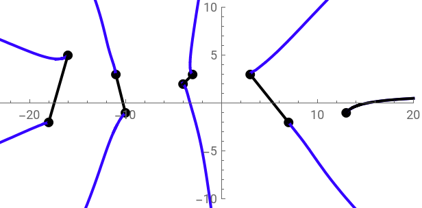
BPPlot=Graphics[Table[{PointSize[Large],Point[{Re[BPs[[k]]],Im[BPs[[k]]]}]},{k,1,Length[BPs]}],Axes->True,PlotRange{{-20,20},{-15,15}}];BPcutsM=Table[Graphics[{Thick,Line[{{Re[BPs[[2k-1]]],Im[BPs[[2k-1]]]},{Re[BPs[[2k]]],Im[BPs[[2k]]]}}]}],{k,1,genus}];BPcuts=Join[BPcutsM,{Graphics[{Thick,Line[{{Re[BPs[[2genus+1]]],Im[BPs[[2genus+1]]]},{20,-0.4}}]}]}];ZeroArg=ContourPlot[Arg[Poly[Rex+IImx]]==0,{Rex,-25,20},{Imx,-15,15},ContourStyle->{Thick,RGBColor[0.2,0,1]}];LCut=ContourPlot[Arg[Poly[Rex+IImx]]==0,{Rex,Re[BPs[[-1]]],20},{Imx,Im[BPs[[-1]]]-5,Im[BPs[[-1]]]+5},ContourStyle->{Thick,Black}];CutPlot=Show[BPPlot,ZeroArg,BPcutsM,LCut,PlotRange->{{-23,20},{-10,10}}]
Out[]=
First and Second Kind Periods
First and Second Kind Periods
First Kind Integrals
First Kind Integrals

In[]:=
PolyRoot[x_]:=;
Abs[Poly[x]]
Exp[IIf[Arg[Poly[x]]<0,Arg[Poly[x]]/2+Pi,Arg[Poly[x]]/2]];dU=Dif1K
-2PolyRoot[x]
In[]:=
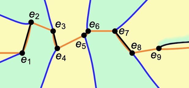
AMapMInf=NIntegrate[dU,{x,-∞,BPs[[1]]},WorkingPrecision18];AMapSet=Table[NIntegrate[dU,{x,BPs[[i]],BPs[[i+1]]},WorkingPrecision18],{i,1,Length[BPs]-1}];AMapPInf=NIntegrate[dU,{x,BPs[[-1]],∞},WorkingPrecision18];AMapSign={-1,-1,-1,1,-1,-1,-1,1};
In[]:=
(ClpsC1=Sum[AMapSet[[2i-1]]AMapSign[[2i-1]],{i,1,genus}]+AMapPInf)//Chop(ClpsC2=AMapMInf+Sum[AMapSet[[2i]]AMapSign[[2i]],{i,1,genus}])//Chop
Out[]=
{0,0,0,0}
Out[]=
{0,0,0,0}
In[]:=
Chop[ClpsC1,]Chop[ClpsC1,]Chop[ClpsC2,]Chop[ClpsC2,]
-17
10
-18
10
-16
10
-17
10
Out[]=
{0,0,0,0}
Out[]=
{8.×+2.×,0,1.06×+1.45×,0}
-18
10
-18
10
-18
10
-18
10
Out[]=
{0,0,0,0}
Out[]=
{7.×-6.×,0,0,0}
-17
10
-17
10
Second Kind Integrals
Second Kind Integrals
First Kind Period Matrices
First Kind Period Matrices
Second Kind Period Matrices
Second Kind Period Matrices
Legendre Relations
Legendre Relations
Verification
Verification
In[]:=
(*ThefunctionwhichcomputesapointoftheJacobianvarietyfromachracteristicCh*)Char2U[Ch_]:=Module[{tCh=Mod[Ch,2]},Sum[tCh[[2,i]]MωA[[All,i]],{i,1,genus}]+Sum[tCh[[1,i]]MωPA[[All,i]],{i,1,genus}]]InvMωA=Inverse[MωA];Acc=5;
Theta Function
Theta Function
Bolza Formula
Bolza Formula
Computation of ℘ - Functions
Computation of ℘ - Functions
KCh=
;
1 | 1 | 1 | 1 |
0 | 1 | 0 | 1 |
℘ - Functions
℘ - Functions
Jacobi inversion problem on branch points
Jacobi inversion problem on branch points
Jacobi inversion problem on arbitrary points
Jacobi inversion problem on arbitrary points
JIP: Example 1a
JIP: Example 1a
◼
Points
◼
Entire rational functions from coordinates
◼
Abel image of D and ℘-functions
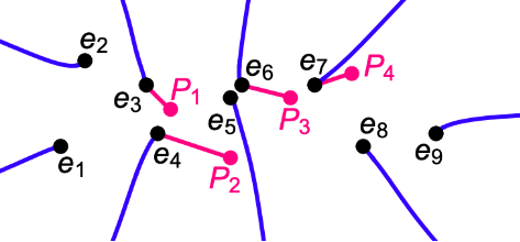
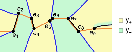
Allarechosenwithsigns=+1Signsofy=±
P
i
(x)
are{1,-1,-1,-1,1,-1,-1,-1,1,1}.Thensign: | real | onSheet1 |
P 1 | + | + |
P 2 | + | + |
P 3 | + | - |
P 4 | + | + |
In[]:=
uP1=AMapMInf+Sum[AMapSet[[i]]AMapSign[[i]],{i,1,2}]+NIntegrate[dU,{x,BPs[[3]],xPs[[1]]},WorkingPrecision18];uP2=AMapMInf+Sum[AMapSet[[i]]AMapSign[[i]],{i,1,3}]+NIntegrate[dU,{x,BPs[[4]],xPs[[2]]},WorkingPrecision18];uP3=-(AMapMInf+Sum[AMapSet[[i]]AMapSign[[i]],{i,1,5}]-NIntegrate[dU,{x,BPs[[6]],xPs[[3]]},WorkingPrecision18]);uP4=AMapMInf+Sum[AMapSet[[i]]AMapSign[[i]],{i,1,6}]+NIntegrate[dU,{x,BPs[[7]],xPs[[4]]},WorkingPrecision18];uP=uP1+uP2+uP3+uP4
Out[]=
{-1.18274997428733205+0.20563451583301787,0.073714132420250436-0.038375141967611938,-0.0047619330249629105+0.0026738674813980292,0.00059219099437290674-0.00006414985341453584}
JIP: Example 1b
JIP: Example 1b
CITE THIS NOTEBOOK
CITE THIS NOTEBOOK
Uniformization of a genus 4 hyperelliptic curve with arbitrary complex branch points
by Julia Bernatska
Wolfram Community, STAFF PICKS, August 8, 2024
https://community.wolfram.com/groups/-/m/t/3243472
by Julia Bernatska
Wolfram Community, STAFF PICKS, August 8, 2024
https://community.wolfram.com/groups/-/m/t/3243472