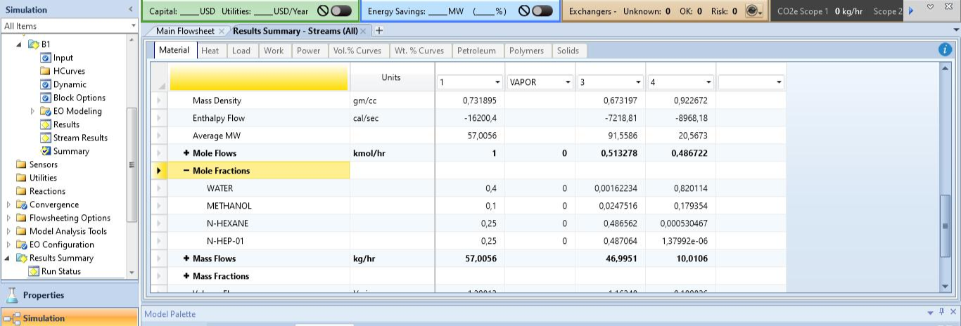
The liquid–liquid equilibrium (LLE) behavior of the quaternary system water (1) + methanol (2) + n-hexane (3) + n-heptane (4) is investigated at 298.15 K using the Non-Random Two-Liquid (NRTL) model with temperature-dependent interaction parameters (reported in Aspen-Plus v.14).
The feed composition considered is:
* Water = 0.40
* Methanol = 0.10
* n-Hexane = 0.25
* n-Heptane = 0.25
The feed composition considered is:
* Water = 0.40
* Methanol = 0.10
* n-Hexane = 0.25
* n-Heptane = 0.25
The equilibrium phase compositions were determined by applying the Common Tangent Hyperplane (CTH) Approach. The calculated compositions of the coexisting liquid phases were:
Liquid Phase 1 (water-rich phase)
Water = 0.820114
Methanol = 0.179354
n-Hexane = 0.000530
n-Heptane = 0.000002
Liquid Phase 2 (hydrocarbon-rich phase)
Water = 0.001622
Methanol = 0.024752
n-Hexane = 0.486562
n-Heptane = 0.487064
Liquid Phase 1 (water-rich phase)
Water = 0.820114
Methanol = 0.179354
n-Hexane = 0.000530
n-Heptane = 0.000002
Liquid Phase 2 (hydrocarbon-rich phase)
Water = 0.001622
Methanol = 0.024752
n-Hexane = 0.486562
n-Heptane = 0.487064
The calculated phase fraction was β = 0.486722, indicating that approximately 48.7% of the overall mixture forms the water-rich phase, while the remaining 51.3% forms the hydrocarbon-rich phase.
The results show a pronounced separation between the polar components (water and methanol) and the nonpolar hydrocarbons (n-hexane and n-heptane). These findings demonstrate the effectiveness of combining CTH analysis with the NRTL model for predicting phase splitting and equilibrium compositions in multicomponent partially miscible systems.
Mathematica results show excellent agreement with their counterparts obtained using Aspen-Plus.
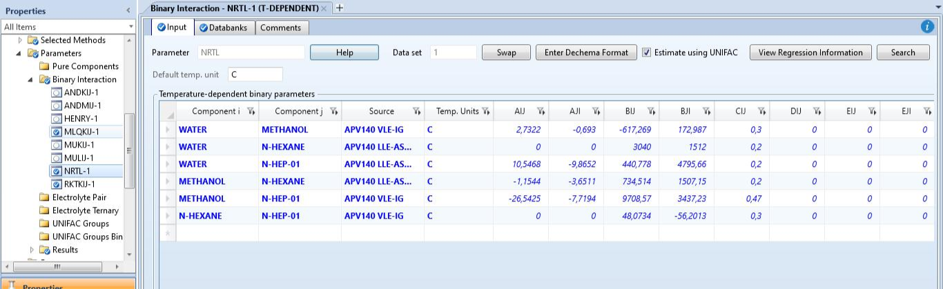
NRTL Parameters from Aspen Plus APV140
Source: Binary Interaction NRTL-1 (T-Dependent)
Convention: tau_ij = Aij + Bij / T(K)
alpha_ij = CIJ (constant)
Component order: 1=Water 2=Methanol 3=n-Hexane 4=n-Heptane
Source: Binary Interaction NRTL-1 (T-Dependent)
Convention: tau_ij = Aij + Bij / T(K)
alpha_ij = CIJ (constant)
Component order: 1=Water 2=Methanol 3=n-Hexane 4=n-Heptane
Aij matrix (rows=i, cols=j)
aNRTL={{0,2.7322,0,10.5468},(*Water*){-0.693,0,-1.1544,-26.5425},(*Methanol*){0,-3.6511,0,0},(*n-Hexane*){-9.8652,-7.7194,0,0}(*n-Heptane*)};
Bij matrix (K)
bNRTL={{0,-617.269,3040,440.778},{172.987,0,734.514,9708.57},{1512,1507.15,0,48.0734},{4795.66,3437.23,-56.2013,0}};
alphaNRTL (CIJ) — symmetric
alphaNRTL={{0,0.30,0.20,0.20},{0.30,0,0.20,0.47},{0.20,0.20,0,0.30},{0.20,0.47,0.30,0}};
Core functions
tauMatrix[T_]:=aNRTL+bNRTL/T;gMatrix[T_]:=Exp[-alphaNRTL*tauMatrix[T]];lnGammaNRTL[x_List,T_?NumericQ]:=Module[{tau=tauMatrix[T],G=gMatrix[T],n=4},Table[Module[{num1,den1,s2},num1=Sum[x[[j]]tau[[j,i]]G[[j,i]],{j,1,n}];den1=Sum[x[[k]]G[[k,i]],{k,1,n}];s2=Sum[Module[{dj=Sum[x[[k]]G[[k,j]],{k,1,n}],nj=Sum[x[[m]]tau[[m,j]]G[[m,j]],{m,1,n}]},x[[j]]G[[i,j]]/dj(tau[[i,j]]-nj/dj)],{j,1,n}];num1/den1+s2],{i,1,n}]];gammaNRTL[x_List,T_?NumericQ]:=Exp[lnGammaNRTL[x,T]];
In[]:=
T=298.15;
NRTL excess Gibbs energy
gE[x_List]:=Module[{s1},s1=Sum[x[[i]](Sum[tauMatrix[T][[j,i]]gMatrix[T][[j,i]]x[[j]],{j,4}]/Sum[gMatrix[T][[k,i]]x[[k]],{k,4}]),{i,4}];s1];
Total dimensionless Gibbs energy
g/RT
g/RT
gMix[x1_,x2_,x3_]:=Module[{x4,x},x4=1-x1-x2-x3;x={x1,x2,x3,x4};Sum[x[[i]]Log[x[[i]]],{i,4}]+gE[x]];
Symbolic gradient
grad=Table[D[gMix[x1,x2,x3],var],{var,{x1,x2,x3}}];
Unknown phase compositions
xa={xa1,xa2,xa3};xb={xb1,xb2,xb3};
Gibbs energies
gA=gMix[xa1,xa2,xa3];gB=gMix[xb1,xb2,xb3];
Gradients
gradA=grad/.{x1->xa1,x2->xa2,x3->xa3};gradB=grad/.{x1->xb1,x2->xb2,x3->xb3};
Common tangent hyperplane equations
eqSlope=Thread[gradA==gradB];eqIntercept=gA-xa.gradA==gB-xb.gradB;
Feed composition
z={0.40,0.10,0.25,0.25};
Phase fractions is beta
Mass balances
eqMB={z[[1]]==(1-beta)xa1+betaxb1,z[[2]]==(1-beta)xa2+betaxb2,z[[3]]==(1-beta)xa3+betaxb3};
Complete system
eqns=Join[eqSlope,{eqIntercept},eqMB];
Solution using FindRoot
sol=FindRoot[eqns,{{xa1,0.82},{xa2,0.18},{xa3,0.0003},{xb1,0.0016},{xb2,0.025},{xb3,0.48},{beta,0.50}},AccuracyGoal->12,PrecisionGoal->12,MaxIterations->1000]//Chop
Out[]=
{xa10.820114,xa20.179354,xa30.000530465,xb10.00162235,xb20.0247519,xb30.486562,beta0.513278}
CITE THIS NOTEBOOK
CITE THIS NOTEBOOK
Phase splitting in a quaternary system by the common tangent hyperplane approach
by Siwar Labidi and Housam Binous
Wolfram Community, STAFF PICKS, June 12, 2026
https://community.wolfram.com/groups/-/m/t/3732706
by Siwar Labidi and Housam Binous
Wolfram Community, STAFF PICKS, June 12, 2026
https://community.wolfram.com/groups/-/m/t/3732706