Abstract
Abstract
The study of cellular automata is useful for modeling many evolving systems. A novel variant of cellular automata that uses sequential updating with multiple sets of rules, resulting in multiway sequential cellular automata, is examined. This structure has the potential for modeling many aspects of quantum mechanics including possibly quantum spin chains. This study examines the 216 possible 2 block sequential updating cellular automata which preserve the identity transformation. The geometric structure of this family of cellular automata is classified into 3 predominant classes differentiated by density and overarching behavior. A deeper exploration is made of particular structures of interest, highlighting the impact of specific subsets of multiway circular sequential cellular automata rules on the directionality, behavior, symmetry, and causal invariance of the resulting states graphs.
Introduction
Introduction
The Quantum World
The Quantum World
Quantum field theory (QFT) studies the theoretical synthesis of classical field theory, special relativity, and quantum mechanics to model the physical behavior of subatomic particles as well as quasi-particles in condensed matter physics. [5] A fundamental aspect of quantum physics is its non-deterministic nature, which stems from Heisenberg's uncertainty principle. A common example of the difference between deterministic classical physics and non-deterministic quantum physics is the comparison of Bohr's model of the atom, which predicts the structure of an atom from a classical standpoint, and the Electron Cloud Model that incorporates the uncertainty of the position and momentum of an electron.
Similar to the model of an atom, both classical and quantum models of physical mechanics are essential to enhancing our understanding of the universe. This exploration aims to model the non-deterministic nature of quantum mechanics using multiway sequential cellular automata.
Similar to the model of an atom, both classical and quantum models of physical mechanics are essential to enhancing our understanding of the universe. This exploration aims to model the non-deterministic nature of quantum mechanics using multiway sequential cellular automata.
Multiway Sequential Cellular Automata
Multiway Sequential Cellular Automata
Cellular automata (CA) are grids of cells defined by an initial state and a list of evolutionary rules. The initial state is a row of black and white cells (2 possible states) of any length. CA rules define how a block of "input" black and white cells are transformed into a new block of different "output" black and white cells. New rows are created by applying these rules to blocks of cells of the rule "input" length. As such, for CA, a "generation of evolution" is a single row.
Sequential CA differ from standard CA in the application of rules on the current state. For sequential CA, blocks of cells to which the rules are applied overlap by 1 or more cells and for each row, only 1 block of cells is transformed while the rest of the cells remain constant. Thus, for sequential CA, a "generation of evolution" consists of several rows. This method of evolution allows the evolution of cells at the beginning of a row to influence the evolution of later cells.
Additional nuance can be added to sequential CA through the use of multiway rules. Multiway CA evolve according to 2 or more sets of rules. Thus, for any given state, there may be several different possible outcomes. These different evolutionary paths can be represented in a multiway graph.
Multiway Circular Sequential Cellular Automata
Multiway Circular Sequential Cellular Automata
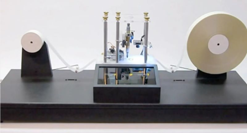
Multiway sequential CA can be implemented with a multiway Turing machine. Turing machines comprise of a "tape" of black and white cells, a black teardrop symbol, the "head," which is located in a cell along the tape, and a set of rules that dictate the actions of the head. Below is an example of a physical Turing machine. [4]
The Turing machine has 3 functions: the head can alter the color of the current cell, the head can move 1 cell to the right or left, and the head can change orientation between up and down. Turing machine rules define a specific cell color change, head movement to the left or right, and the new orientation of the head for every possible configuration of current orientation of the head and current cell color. An example of a set of Turing machine rules is below.
In[]:=
RulePlot[TuringMachine[100]]
Out[]=
For multiway Turing machines, there are 2 or more sets of Turing machine rules which allow the Turing machine to evolve in different ways. Like multiway CA, these various paths of evolution can be organized into a multiway graph.
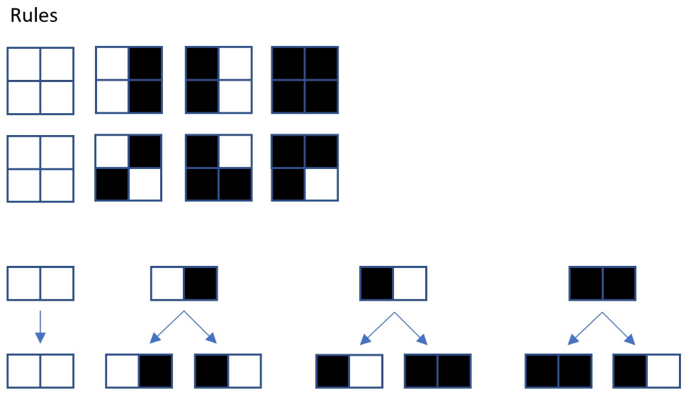
The attributes of multiway Turing machines are compatible with multiway sequential CA which use rules that transform blocks of 2 cells into blocks of 2 new cells. The value of a cell and the head's orientation each store 1 bit of information; as such, a 2 cell block can be represented with these 2 attributes. The sequential nature of the CA studied can be modeled with the movement of the head 1 cell to the right after each rule-informed transformation of the tape. A visualization of this implementation of multiway sequential CA using a multiway Turing machine is below. The rules are defined as follows (shown in 2 ways).
The attributes of multiway Turing machines are compatible with multiway sequential CA which use rules that transform blocks of 2 cells into blocks of 2 new cells. The value of a cell and the head's orientation each store 1 bit of information; as such, a 2 cell block can be represented with these 2 attributes. The sequential nature of the CA studied can be modeled with the movement of the head 1 cell to the right after each rule-informed transformation of the tape. A visualization of this implementation of multiway sequential CA using a multiway Turing machine is below. The rules are defined as follows (shown in 2 ways).
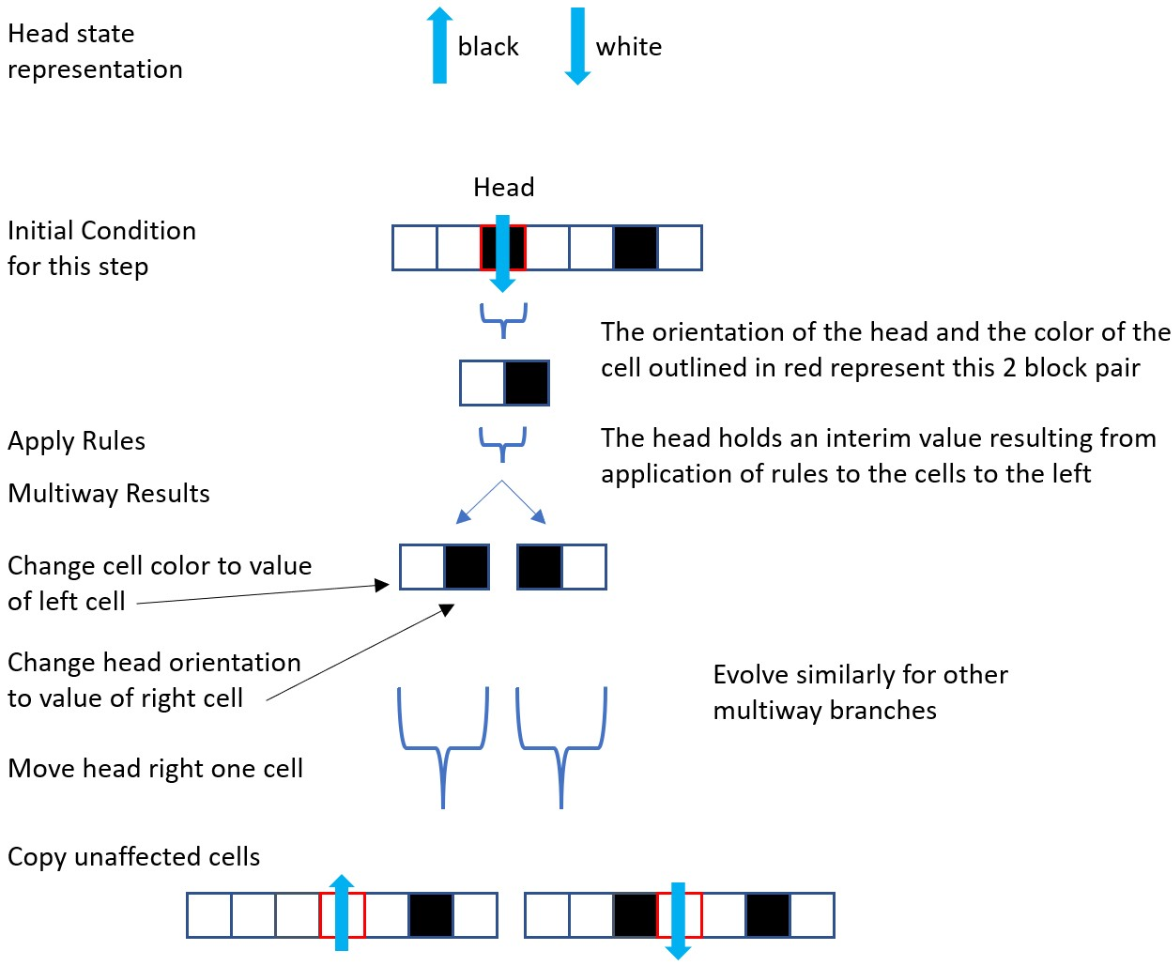
An interesting consequence of this model is that the cells at the end of each row in fact influence the cells at the beginning of the row in the next generation. This behavior can be called multiway circular sequential CA (MCSCA). This structure has the potential to model many quantum phenomena such as quantum spin chains.
Evolutionary Graphs
Evolutionary Graphs
M-type MCSCA Rules
M-type MCSCA Rules
The M-type rules particular to this study each consist of 2 complete sets of CA rules. As such, these multiway M-type rules define 2 possible outcomes for each state. Each box of 4 black and white squares in the visual displays of these rules, such as in the diagrams below, represents a single transformation from the input state, specified by the 2 black and white squares in the first row, to the output block of 2 cells, which is displayed in the second row.
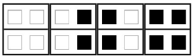
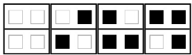
All M-type rules transform 2 white squares into 2 white squares to preserve an “identity” transformation.
To create a comprehensive list of rules, a list of all possible combinations of inputs and outputs is generated:
In[]:=
possibles=Flatten[Table[{{a,b},{c,d}},{a,{0,1}},{b,{0,1}},{c,{0,1}},{d,{0,1}}],3]
Out[]=
{{{0,0},{0,0}},{{0,0},{0,1}},{{0,0},{1,0}},{{0,0},{1,1}},{{0,1},{0,0}},{{0,1},{0,1}},{{0,1},{1,0}},{{0,1},{1,1}},{{1,0},{0,0}},{{1,0},{0,1}},{{1,0},{1,0}},{{1,0},{1,1}},{{1,1},{0,0}},{{1,1},{0,1}},{{1,1},{1,0}},{{1,1},{1,1}}}
These rules are then partitioned into rules with input of white black (0,1), black white (1,0), and black black (1,1).
The following lists contain all possible combinations of 2 outputs for each input to create the multiway aspect of the rule system:
In[]:=
wb=Subsets[Partition[possibles,4][[2]],{2}]
Out[]=
{{{{0,1},{0,0}},{{0,1},{0,1}}},{{{0,1},{0,0}},{{0,1},{1,0}}},{{{0,1},{0,0}},{{0,1},{1,1}}},{{{0,1},{0,1}},{{0,1},{1,0}}},{{{0,1},{0,1}},{{0,1},{1,1}}},{{{0,1},{1,0}},{{0,1},{1,1}}}}
In[]:=
bw=Subsets[Partition[possibles,4][[3]],{2}]
Out[]=
{{{{1,0},{0,0}},{{1,0},{0,1}}},{{{1,0},{0,0}},{{1,0},{1,0}}},{{{1,0},{0,0}},{{1,0},{1,1}}},{{{1,0},{0,1}},{{1,0},{1,0}}},{{{1,0},{0,1}},{{1,0},{1,1}}},{{{1,0},{1,0}},{{1,0},{1,1}}}}
In[]:=
bb=Subsets[Partition[possibles,4][[4]],{2}]
Out[]=
{{{{1,1},{0,0}},{{1,1},{0,1}}},{{{1,1},{0,0}},{{1,1},{1,0}}},{{{1,1},{0,0}},{{1,1},{1,1}}},{{{1,1},{0,1}},{{1,1},{1,0}}},{{{1,1},{0,1}},{{1,1},{1,1}}},{{{1,1},{1,0}},{{1,1},{1,1}}}}
Complete M-type rules are derived below from these combinations of 2 possible outputs for the 3 cases of black and white cells:
In[]:=
rules=Flatten[Table[Join[{{{0,0},{0,0}},{{0,0},{0,0}}},x,y,z],{x,wb},{y,bw},{z,bb}],2];
Each rule is then re-ordered into a list of 2 complete sets of rules:
In[]:=
caRules=Table[{n[[{1,3,5,7}]],n[[{2,4,6,8}]]},{n,rules}];
Each sublist in the above list is one complete M-type rule. There are 216 possible combinations of input to output rules such that there are 2 distinct outputs for every possible input and the identity is preserved for white-white mapping to white-white. Rules M1 to M216 are examined in this study.
States Graphs
States Graphs
States graphs display the relationships between all possible states of the cellular automaton. Each node of the states graph represents a distinct state of the MCSCA while the edges of the graph represent the application of a M-type rule to transform one state to another. States graphs can be calculated for any step of the MCSCA's evolution.
Below is an example of a states graph after 5 steps of evolution:
In[]:=
tmRule95={{{2,0}{2,0,1},{2,1}{2,0,1},{1,0}{1,0,1},{1,1}{1,0,1}},{{2,0}{2,0,1},{2,1}{1,1,1},{1,0}{2,1,1},{1,1}{1,1,1}}};ResourceFunction["MultiwayTuringMachine"][tmRule95,{{2,1,0},{0,1,0,1,1}},5,"StatesGraph",VertexSize->1]
Out[]=
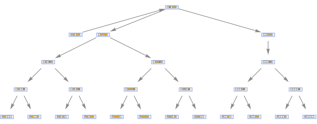
As the number of steps of evolution increases, the density of the graph increases meaning that the states that were displayed at the nodes in the above graph are now represented by blue points.
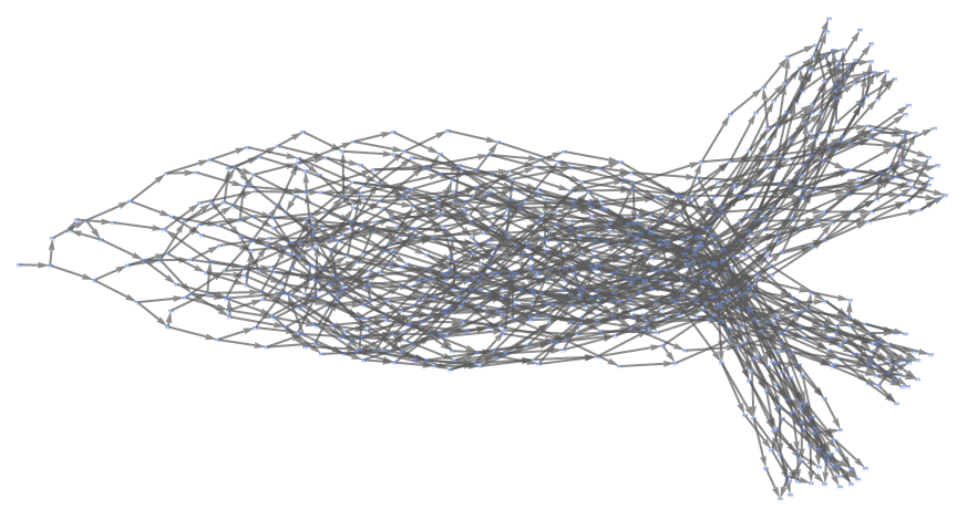
A states graph displaying the 20th step of evolution was generated using the same initial condition for all 216 possible M-type rules. Below is an example of one such graph.
Out[]=
Graph Classes
Graph Classes
The 216 graphs can be broadly classified into 4 classes of graphs.
Class 1 Graphs
Class 1 Graphs
Class 1 graphs resemble the shape of a squid, with a peak at one end and several tendrils emitting from the opposite end in a circular manner. Within Class 1 graphs, there are 2 sub-categories: right-pointing "squid" graphs and left-pointing "squid" graphs as shown below.
The evolution of a states graph can be further clarified by viewing the graph after each individual step of evolution. Note that n represents the number of evolutionary steps.
To view the overall trend of evolution, a states graph is shown for a right-facing "squid" after 100 evolutionary steps.
A complete table of all the Class 1 graphs is below, split into right and left-facing "squid."
Class 2 Graphs
Class 2 Graphs
Class 2 graphs are sparse and are made of several intertwined circular behaviors. An example of a class 2 graph is shown below.
The evolution of this graph can also be displayed step-by-step as follows:
The figure below shows the states graph after 100 evolutionary steps.
A complete table of all the Class 2 graphs is below.
Class 3 Graphs
Class 3 Graphs
While Class 1 and 2 graphs are the most common, there are several graphs that extend outwards from a central circular shape in several directions—these graphs belong to Class 3. An example of a Class 3 graph is shown below.
The evolution of this graph can also be displayed step-by-step as follows:
The graph below is the states graph after evolving for 100 steps.
A complete table of all the Class 3 graphs is below.
Class 4 Graphs
Class 4 Graphs
There are 5 pairs of special cases that are grouped into Class 4 as they have unique characteristics.
◼
The first pair has a lattice structure.
◼
The second has a body similar to graphs of Class 1 but has a long tail feature.
◼
The third pair resembles graphs of Class 3 but without the extended "arms".
◼
The fourth pair resembles both Classes 1 and 3.
◼
The final (fifth) pair is very similar to Class 1 graphs but with a Class 2 attribute overlayed.
The evolution of these graphs can also be displayed step-by-step:
The graphs below are the states graphs after 100 evolutionary steps for the first, second, and third types of Class 4 graphs, respectively.
Graph Analysis
Graph Analysis
1
.Close examination of the directionality of Class 1 graphs shows that the rule governing the output of a white-black block can flip the direction of the graph from left-facing to right-facing. If the rule is white-black to white-black, the graph is left-facing. If the rule is white-black to black-black, the graph is right-facing by generation 20. Further examination of the data is needed to determine whether this directionality converges in all cases.
2
.Symmetry is an important characteristic to study in graph analysis. It was found here that symmetrical “squid,” such as the graph produced by rule M173, only have the outputs white-black or black-black. Hence, the duality of the outputs leads to graphical symmetry.
3
.A detailed exploration of Class 2 graphs reveals a complementary situation to that of Class 1 graphs. All Class 2 graphs are found to have emanated from the application of rules that map black-white to a 2 block structure with a white block on the left. In Class 1 graphs, it was found that the mapping of the white-black block determined directionality based on the resulting left block. Similarly, the left block resulting from the application of rules to the complement, the black-white 2 block structure, governs the Class 2 structure. The greater impact of the left block over the right block in both of these cases is due to the structure of the algorithm employed. The right block that results from the rules is essentially an intermediate value and, as such, has less direct impact on the resulting graph.
4
.Another interesting characteristic to examine is causal invariance, the preservation of events and causation through all possible evolutionary routes through the multiway graph. In the MCSCA case, this yields interesting results. All of the Class 1, 2, and 3 samples tested were causal invariant unlike the group of Class 4 graphs tested, for which only some were causal invariant.
5
.Lastly, there is some structural similarity in all of the graphs that have evolved to 100 steps. However, inherent differences still persist between graphs of the different classes.
Conclusion and Future Work
Conclusion and Future Work
A novel form of cellular automata, multiway circular sequential cellular automata, was studied. This form of CA has the potential for modeling systems such as quantum spin chains where states in a system have effects that propagate beyond their immediate neighbors. In studying the evolution of MCSCA, it was found that the graphs fell into 3 predominant classes separated by their form and density. Particular bits of the MCSCA rules were found to play a role in determining directionality and structure. Symmetry and causal invariance of these classes of graphs were also examined.
For a more complete understanding of MCSCA, more research is needed into the effects of varying initial conditions and the application of probabilistic rules to enable study of the non-deterministic MCSCA. The development of quantitative measures to compare graphs as well as to analyze the recurrence rates of states as generations progress would be valuable.
For a more complete understanding of MCSCA, more research is needed into the effects of varying initial conditions and the application of probabilistic rules to enable study of the non-deterministic MCSCA. The development of quantitative measures to compare graphs as well as to analyze the recurrence rates of states as generations progress would be valuable.
Acknowledgements
Acknowledgements
I would like to thank Stephen Wolfram for the opportunity to work on this project. I would also like to thank Adiba Shaikh for her continual support throughout my work. James Boyd, Michael Trott, and Peter Barendse also provided extremely valuable technical discussions.
References
References
1
.Boyd, J. (2022, June 6). Multicomputational Irreducibility. Wolfram Physics Project. https://www.wolframphysics.org/bulletins/2022/06/multicomputational-irreducibility/
2
.3
.Gorard, J. MultiwayTuringMachine. Wolfram Function Repository. https://resources.wolframcloud.com/FunctionRepository/resources/MultiwayTuringMachine/
4
.Guizzo, E. (2010, March 26). DIY Turing Machine. IEEE Spectrum. https://spectrum.ieee.org/032610-diy-turing-machine
5
.Peskin, M. E., Schroeder, D. (1995). An Introduction to Quantum Field Theory (Avalon Publishing)
6
.Wolfram, S. (2002). A New Kind of Science. Wolfram Media.
7
.Wolfram, S. (2020, June 9). Exploring Rulial Space: The Case of Turing Machines. Wolfram Physics Project. https://www.wolframphysics.org/bulletins/2020/06/exploring-rulial-space-the-case-of-turing-machines/#the-cellular-automaton-analog
8
.Wolfram, S. (2021, February 4). Multiway Turing Machines. Wolfram Physics Project. https://www.wolframphysics.org/bulletins/2021/02/multiway-turing-machines/