Ponchon-Savarit Diagram for an Ethanol-Water Binary Mixture
Authors: Housam Binous and Ahmed Bellagi
Ponchon-Savarit Diagram for an Ethanol-Water Binary Mixture
Authors: Housam Binous and Ahmed Bellagi
Authors: Housam Binous and Ahmed Bellagi
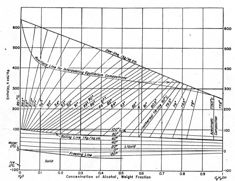
The Ponchon–Savarit diagram provides a graphical method for solving coupled material and energy balances in separation processes involving binary mixtures. Here, we illustrate how the Ponchon–Savarit diagram can be computed for a non-ideal binary mixture that has an azeotrope.Consider a binary mixture of ethanol and water at atmospheric pressure. The gas phase is assumed ideal, but the liquid phase is non-ideal. We plot the Ponchon–Savarit diagram, which is also called the enthalpy-composition diagram. Enthalpy is expressed in kcal/kg and composition is expressed in weight fraction of ethanol. Also shown is the vapor equilibrium curve for ethanol-water.Enthalpies for the liquid and vapor phases are computed using the following equations:(,T)=(T-)+(1-)(T-)+,(,T)=[+(T-)]+(1-)[+(T-)],where is the latent heat of vaporization of chemical species at =273.15Kelvin and and are the heat capacities for the liquid and the gas phases of chemical species , respectively; is a slowly-varying function of temperature and can be assumed constant [3]. The mole fractions of ethanol in the liquid and gas phases are denoted by and , respectively. Finally, is the excess enthalpy, which accounts for the non-ideal behavior of the liquid mixture. We use the following correlation from [2] to compute the excess enthalpy as a function of composition and temperature: =(1-)(T)+(T)+(T)+(T)+(T), where is the mixture temperature and is the ethanol mole fraction. Here, (T)=+T+, where and , , and are appropriate constants tabulated in [2].The Ponchon–Savarit diagram for closely agree with Figure 2-4 in [1] given below:Finally, the "tie lines", displayed in green, show the composition of the two phases that exist in equilibrium at the specified temperature. At the azeotropic composition the tie line is shown in red; it is vertical, confirming that = at the azeotrope. At , the azeotrope composition in terms of ethanol weight fraction is 96% and the boiling temperature is .We compare out results to the digitized data of the Figure given above.
H
L
x
ethanol
x
ethanol
C
P,L,ethanol
T
ref
x
ethanol
C
P,L,water
T
ref
E
H
H
V
y
ethanol
y
ethanol
λ
ethanol
C
P,V,ethanol
T
ref
y
ethanol
λ
water
C
P,V,water
T
ref
λ
i
i
T
ref
C
P,L,i
C
P,V,i
i
λ
i
x
ethanol
y
ethanol
E
H
E
H
x
ethanol
x
ethanol
a
0
a
0.5
0.5
x
ethanol
a
1.5
1.5
x
ethanol
a
2.5
2.5
x
ethanol
a
4.5
4.5
x
ethanol
T
x
ethanol
a
m
b
m
c
m
d
m
2
T
m=0,0.5,1.5,2.5,4.5
b
m
c
m
d
m
P=760mmHg
x
ethanol
y
ethanol
P=760mmHg
T=78.16°C
References:
[1] P. C. Wankat, Separation Process Engineering, 3rd ed., Upper Saddle River, NJ: Pearson, 2012.
[2] J. A. Larkin, "Thermodynamic Properties of Aqueous Non-Electrolyte Mixtures I. Excess Enthalpy for Water + Ethanol at 298.15 to 383.15 K," Journal of Chemical Thermodynamics, 7(2), 1975 pp. 137–148.
[3] R. H. Perry and D. W. Green, Perry's Chemical Engineers' Handbook, 7th ed., New York: McGraw–Hill, 1997.
Total pressure in mmHg
In[]:=
P=760;
Antoine Constants and equation for ethanol and water.
In[]:=
Aa1=7.68117;Ba1=1332.04;Ca1=199.200;Aa2=8.07131;Ba2=1730.63;Ca2=233.426;Psat1=10^(Aa1-Ba1/(T+Ca1));Psat2=10^(Aa2-Ba2/(T+Ca2));
Binary interaction parameters for the Van Laar activity coefficient model
In[]:=
A12=1.66480;A21=0.94010;Gam1[xa_]:=Exp[A12(A21(1-xa)/(A12xa+A21(1-xa)))^2];Gam2[xa_]:=Exp[A21(A12xa/(A21(1-xa)+A12xa))^2];
Computing VLE data for the binary system: Ethanol and Water
In[]:=
i=0;While[i<1001,{xa=i0.001,sol=FindRoot[Psat1xaGam1[xa]+Psat2(1-xa)Gam2[xa]P,{T,77,78}];xe[i]=xa,ye[i]=Psat1xaGam1[xa]/P/.sol,Te[i]=T/.sol,i++}];Tbl1=Table[{xe[i],Te[i]},{i,0,1000}];Tbl2=Table[{ye[i],Te[i]},{i,0,1000}];Tbl3=Table[{xe[i],ye[i]},{i,0,1000}];Tx=Interpolation[Tbl1,InterpolationOrder1];Ty=Interpolation[Tbl2,InterpolationOrder1];xy=Interpolation[Tbl3,InterpolationOrder1];solaz=FindRoot[xy[t]t,{t,0.9}];(*latentheatofvaporization.SeeRef.3*)C1A=5.690010^7;C2A=0.3359;C3A=0;C4A=0;C1B=5.205310^7;C2B=0.3199;C3B=-0.212;C4B=0.25795;TcA=513.92;TcB=647.13;λA=10^-3C1A(1-Ti2/TcA)^(C2A+C3ATi2/TcA+C4A(Ti2/TcA)^2);λB=10^-3C1B(1-Ti2/TcB)^(C2B+C3BTi2/TcB+C4B(Ti2/TcB)^2);Ti2=0+273.15;H[y_]:=y(λA+73.98(Ty[y]))+(1-y)(λB+38.29(Ty[y]));(*vapor-phaseenthalpy*)h[x_]:=x(118.1(Tx[x]))+(1-x)(75.66(Tx[x]))+x(1-x)(a0+a1x^0.5+a2x^1.5+a3x^2.5+a4x^4.5);(*liquid-phaseenthalpy*)(*excessenthalpyasafunctionofcompositionandtemperatureisadded.SeeRef.2Itisgivenby:x(1-x)(a0+a1x^0.5+a2x^1.5+a3x^2.5+a4x^4.5)*)a0=-3.6386810^5+1.8382910^3(Tx[x]+273.15)-2.32763(Tx[x]+273.15)^2;a1=9.2598210^5-4.8358610^3(Tx[x]+273.15)+6.37228(Tx[x]+273.15)^2;a2=-14.0489410^5+7.5166110^3(Tx[x]+273.15)-10.11280(Tx[x]+273.15)^2;a3=10.9131810^5-5.8949810^3(Tx[x]+273.15)+7.98868(Tx[x]+273.15)^2;a4=-2.7998610^5+1.5055710^3(Tx[x]+273.15)-2.03127(Tx[x]+273.15)^2;Hw[w_]:=H[x]/(18(1-x)+46x)/4.18/.x-;(*vapor-phaseenthalpyinkcal/kg*)hw[w_]:=h[x]/(18(1-x)+46x)/4.18/.x-;(*liquid-phaseenthalpyinkcal/kg*)yw0=xy-;vw0=46yw0/(46yw0+18(1-yw0));w0az=46t/(46t+18(1-t))/.solaz;yw0az=xy-;vw0az=46yw0az/(46yw0az+18(1-yw0az));
9w
-23+14w
9w
-23+14w
9w0
-23+14w0
9w0az
-23+14w0az
Plot of the Ponchon-Savarit diagram at P=760 mmHg.
Tie-lines are given in Green. Dew line and bubble line are in Yellow and Blue. The tie-line for the azeotrope is given in Red.
Tie-lines are given in Green. Dew line and bubble line are in Yellow and Blue. The tie-line for the azeotrope is given in Red.
Plot of the equilibrium curve at P=760 mmHg. The azeotrope is indicated by the Green dot.
Comparing our calculation results and digitized data (shown by red dots) of Figure 2-4 in [1].
Converting weight fraction (digitized data from Fig 2-4 of Ref 1) into mole fractions
Comparing our calculation results and digitized data (shown by red dots) obtained using the tie-lines of Figure 2-4 in [1].