Simulation of the Separation of n-Heptane/Ethyl Benzene Mixture at 101.325 kPa
Authors: Housam Binous and Ahmed Bellagi
Simulation of the Separation of n-Heptane/Ethyl Benzene Mixture at 101.325 kPa
Authors: Housam Binous and Ahmed Bellagi
Authors: Housam Binous and Ahmed Bellagi
Here, we follow an example given in the website (www.msubbu.in), which has chemical engineering class notes and related materials.
Problem statement:
1000 kg/hr of a mixture containing 42 mole percent heptane (C7H16) and 58 mole percent ethyl benzene (C6H5C2H5) is to be fractionated to a distillate containing 97 mole percent heptane and a residue containing 99 mole percent ethyl benzene using a total condenser and feed at its saturated liquid condition .
We will compute using Mathematica©:
1- Minimum reflux ratio
2- Minimum number of stages at total reflux
3- Number of stages at reflux ratio of 2.5
4- Condenser duty
5- Reboiler duty
The enthalpy - concentration data for the heptane - ethyl benzene at 1 atm pressure are determined as follows .
The enthalpy - concentration data for the heptane - ethyl benzene at 1 atm pressure are determined as follows .
Data from the Web: https://msubbu.in/sp/mt/Ponchon-Savarit.htm
In[]:=
data={{"xheptane","yheptane","Hl (kJ/kmol) x 10^3","Hv (kJ/kmol) x 10^-3"},{0.,0.,24.3,61.2},{0.08,0.28,24.1,59.6},{0.18,0.43,23.2,58.5},{0.25,0.51,22.8,58.1},{0.49,0.73,22.05,56.5},{0.65,0.83,21.75,55.2},{0.79,0.90,21.7,54.4},{0.91,0.96,21.6,53.8},{1.0,1.0,21.4,53.3}};
In[]:=
data//TableForm
Out[]//TableForm=
xheptane | yheptane | Hl (kJ/kmol) x 10^3 | Hv (kJ/kmol) x 10^-3 |
0. | 0. | 24.3 | 61.2 |
0.08 | 0.28 | 24.1 | 59.6 |
0.18 | 0.43 | 23.2 | 58.5 |
0.25 | 0.51 | 22.8 | 58.1 |
0.49 | 0.73 | 22.05 | 56.5 |
0.65 | 0.83 | 21.75 | 55.2 |
0.79 | 0.9 | 21.7 | 54.4 |
0.91 | 0.96 | 21.6 | 53.8 |
1. | 1. | 21.4 | 53.3 |
Generating our own data with the help of Aspen-Hysys®.
Total pressure in kPa
In[]:=
P=101.325;
Antoine Constants and equation for heptane and ethyl benzene
In[]:=
A1=13.8622;B1=2910.26;C1=216.432;
In[]:=
A2=13.9726;B2=3259.93;C2=212.300;
In[]:=
Psat1[temp_]:=ExpA1-;(*heptane*)Psat2[temp_]:=ExpA2-;(*ethylbenzene*)
B1
temp+C1
B2
temp+C2
Normal boiling temperatures in °C
In[]:=
FindRoot[Psat1[T]P,{T,60}]
Out[]=
{T98.3995}
In[]:=
FindRoot[Psat2[T]P,{T,60}]
Out[]=
{T136.197}
Computing VLE data for the binary system: Ethanol and Water as well as h-x and H-y data
1- The VLE data is obtained using the Wilson model.
2- h-x and H-y data are obtained using the thermodynamic database of Aspen-Hysys®.
We check our results against their counterparts given in WWW.
1- The VLE data is obtained using the Wilson model.
2- h-x and H-y data are obtained using the thermodynamic database of Aspen-Hysys®.
We check our results against their counterparts given in WWW.
In[]:=
i=0;V1m=0.1477;V2m=0.12295;(*molarvolumes*)l12=127.14;l21=186.111;(*binaryinteractionparametersinkcal/kmol*)A12=V2m/V1mExp[-l12/(Rg*(T+273.15))];A21=V1m/V2mExp[-l21/(Rg*(T+273.15))];Rg=1.987;(*universalgasconstantiskcal/K*kmol*)(*activitycoefficients*)Gam1[xa_]:=Exp[-Log[xa+(1-xa)*A12]+1-(xa/(xa+(1-xa)*A12)+(1-xa)*A21/(xa*A21+(1-xa)))];Gam2[xa_]:=Exp[-Log[xa*A21+(1-xa)]+1-(xa*A12/(xa+(1-xa)*A12)+(1-xa)/(xa*A21+(1-xa)))];While[i<1001,{xa=i0.001,sol=FindRoot[Psat1[T]Gam1[xa]xa+Psat2[T]Gam2[xa](1-xa)P,{T,77,78}];xe[i]=xa,ye[i]=Psat1[T]Gam1[xa]xa/P/.sol,Te[i]=T/.sol,i++}];Tbl1=Table[{xe[i],Te[i]},{i,0,1000}];Tbl2=Table[{ye[i],Te[i]},{i,0,1000}];Tbl3=Table[{xe[i],ye[i]},{i,0,1000}];Tx=Interpolation[Tbl1,InterpolationOrder1];(*bubbletemperaturein°C*)Ty=Interpolation[Tbl2,InterpolationOrder1];(*dewtemperaturein°C*)xy=Interpolation[Tbl3,InterpolationOrder1];(*VLEdata*)
In[]:=
xvalues={0,0.08,0.18,0.25,0.49,0.65,0.79,0.91,1.0};yvalues={0,0.28,0.43,0.51,0.73,0.83,0.90,0.96,1.0};
In[]:=
Style[TableForm[Join[{{"x","T_present","y_present","y_reference"},Transpose@Table[{xvalues[[i]],Tx[xvalues[[i]]],xy[xvalues[[i]]],yvalues[[i]]},{i,1,Length[xvalues]}]}],TableSpacingAutomatic],{16,Darker@Red}]
Out[]=
x | T_present | y_present | y_reference | ||||||||||||||||||||||||||||||||||||
|
|
|
|
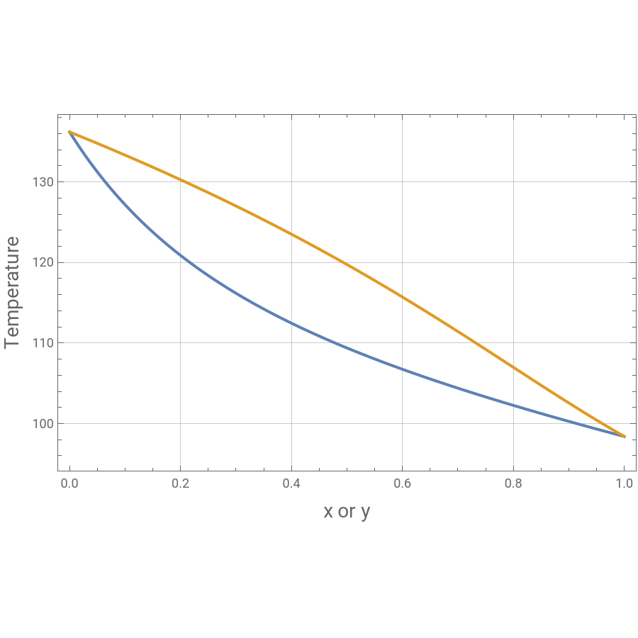
Plotting VLE data for the binary system (heptane/ethyl benzene)
In[]:=
ListPlot[{Tbl1,Tbl2},FrameTrue,GridLinesAutomatic,Joined->True,PlotStyle->Thick,ImageSize450{1,1},FrameLabel{Style["x or y",14],Style["Temperature",14]}]
Out[]=
Computing h-x and H-y data
We have adjusted the reference temperature to 7.25°C in order to match the data given in the following WWW page:
https://msubbu.in/sp/mt/Ponchon-Savarit.htm
We have adjusted the reference temperature to 7.25°C in order to match the data given in the following WWW page:
https://msubbu.in/sp/mt/Ponchon-Savarit.htm
In[]:=
(*purecomponententhalpies-referencestates:h1=h2=0at25°Cand101.325kPa*)A=(0.0+218.5T-0.1484T^2+3.53710^-004T^3+4.71910^-13T^4)/.T(7.25+273.15);hl1=0.0+218.5T-0.1484T^2+3.53710^-004T^3+4.71910^-13T^4-A;B=(0.0+133.2T+2.22510^-2T^2+1.32110^-004T^3+9.95910^-013T^4)/.T(7.25+273.15);hl2=0.0+133.2T+2.22510^-2T^2+1.32110^-004T^3+9.95910^-013T^4-B;Hv1=43100+282.7T-0.7166T^2+1.66310^-003T^3-1.24810^-006T^4-A;Hv2=54320+104.1T-3.20710^-2T^2+2.30110^-004T^3-1.55410^-007T^4-B;(*mixtureenthalpies*)Hvhysys[y_]:=(yHv1+(1-y)Hv2)/.T(Ty[y]+273.15);hlhysys[x_]:=(xhl1+(1-x)hl2)/.T(Tx[x]+273.15);
In[]:=
P2=Plot[{hlhysys[x],Hvhysys[x]},{x,0,1},FrameTrue,FrameLabel{Style["mole fraction of heptane",14],Style["enthalpy kJ / kmole",14]},GridLinesAutomatic,ImageSize{600,350},PlotStyleThick,PlotRange->{{0,1},{10000,65000}},AspectRatio->1.8,ImageSize->500{1,1}]
Plotting h-x and H-y data:
Tie lines are in Green. Dew line and boiling line are in yellow and blue, respectively.
Tie lines are in Green. Dew line and boiling line are in yellow and blue, respectively.
Minimum reflux ratio is equal to 1.17334
Minimum reflux ratio is equal to 1.17334
Minimum number of stages at total reflux = a little more than 7 (obtained using McCabe & Thiele diagram)
Minimum number of stages at total reflux = a little more than 7 (obtained using McCabe & Thiele diagram)
Number of stages at reflux ratio of 2.5
Number of stages at reflux ratio of 2.5
Interpolation to get tie lines
h-x (in blue) and H-y (in yellow) curves with tie lines (in magenta)
Conjugate line (in blue)
h-x and H-y curves with tie lines and conjugate line - a particular tie line (shown in red) is obtained using the conjugate line.
Computing the number of equilibrium stages at total reflux obtained using Ponchon-Savarit diagram.
The condenser is a total condenser. A total of 7 stages are required including the reboiler .
The condenser is a total condenser. A total of 7 stages are required including the reboiler .
We now treat the finite reflux ratio case (i.e., RefuxRatio=2.5).
Stepping off stages in the rectifying section. We change operating line when the equilibrium tie line crosses the line joining the difference points.
The optimum feed stage is stage 6 from the top.
The condenser is a total condenser.
Stepping off stages in the rectifying section. We change operating line when the equilibrium tie line crosses the line joining the difference points.
The optimum feed stage is stage 6 from the top.
The condenser is a total condenser.
Stepping off stages in the stripping section. We change operating line when the equilibrium tie line crosses the line joining the difference points.
The optimum feed stage is stage 6. A total of 11 stages is required including the reboiler.
The optimum feed stage is stage 6. A total of 11 stages is required including the reboiler.
Final Ponchon - Savarit construction