In previous post graph-based model centrality of geometric figure was proposed. Here it suggests similar way of distributing several centroids to an arbitrary (and 3D) regions. This post also contains questions that may be useful to contributors and developers (marked LightRed) so will be grateful for comments and suggestions!
Start of notebook takes 10-12 sec, for running init cells.
Start of notebook takes 10-12 sec, for running init cells.
Introduction
Introduction
Previously was proposed a way for defining unusual, but intuitive clear centroid of region. These points maximize measure for all distances (inside a figure) to boundary:
min
max
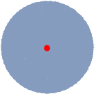

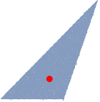
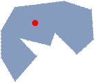
However, for many figures it is only possible to define a certain area of centrality; a single centroid makes no sense:But we can place within the figure several centroids, which in some sense cover the area uniformly. Different ways of generating evenly distributed centers are known: Poisson disk, Centroidal Voronoi tesselation, potential energy minimization etc. But all of them do not work correctly with complex, non-convex figures. The basic idea is to consider the figure as a mesh graph and use the distances on this graph instead of Cartesian coordinates.
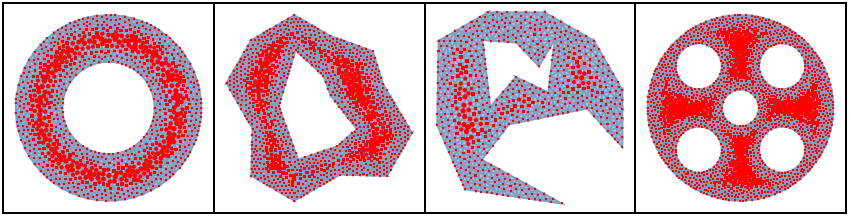
Graph representation of region
Graph representation of region
As in the first post, we will use MeshRegion, MeshConnectivityGraph and GraphDistanceMatrix. I was very impressed with Wolfram Physics Project. It seems that continuous objects just are abstraction, and that the nature of reality is closer to the models proposed in the WPP or Causal Dynamic Triangulation for example. I think sooner or later all theoretical and numerical calculations will become discrete.
Sample of region
For better results MaxCellMeasure should be decreased;
but it will also increase the amount of computing
For better results MaxCellMeasure should be decreased;
but it will also increase the amount of computing
In[]:=
region=DiscretizeRegion[Annulus[],MaxCellMeasure{"Length"0.1},ImageSize->Tiny]
Out[]=

This module take MeshRegion and return:
- Mesh coordinates
- Indices of boundary and interior mesh points (aka graph vertices)
- Mesh connectivity graph
- Distance matrix
To save memory it would be appropriate to use NumericArray, but unfortunately they do not yet support RandomSample, MaximalBy etc. The constant conversion to Normal looks cumbersome. Perhaps there are options for implementation NumericArrays.
In[]:=
Clear[graphFromRegionData];(*For 2D and 3D*)graphFromRegionData[reg_]:=Module[{ coords=MeshCoordinates@reg, graphU=MeshConnectivityGraph[reg,0,AnnotationRulesNone], bound,inter,dm}, {bound,inter}= MeshCellIndex[reg,{0,#}]〚All,2〛 &/@{"Boundary","Interior"}; dm=GraphDistanceMatrix[ Graph[graphU,EdgeWeightTable[eEuclideanDistance[coords〚e〚1〛〛,coords〚e〚2〛〛], {e,EdgeList@graphU}]], Method"Dijkstra"]; <|"indsCoords"->coords,"boundInds"->bound, "interInds"->inter,"graph"->graphU,"distanceMatrix"->dm|>];
Now all computations related to the topology of the region will use direct reference to the vertices of the graph (mesh) rather than to the Cartesian coordinates.
In[]:=
data=graphFromRegionData[region];
In[]:=
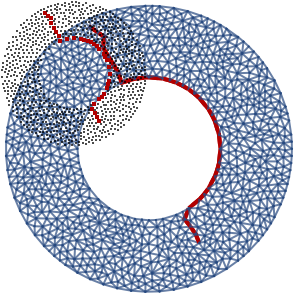
g=Graph[data["graph"],VertexCoordinates->data["indsCoords"],VertexSize->Tiny,ImageSize->150];Row[{HighlightGraph[g,PathGraph[FindShortestPath[g,103,305]],GraphHighlightStyle"Thick"],data["distanceMatrix"]〚103,305〛}]
Out[]=
2.04202
3D regions are... simplest case?
3D regions are... simplest case?
If the figure has no free (open) edges (and this is true for so many 3D forms), we can formulate a goal function for centroids configuration using only the relative positions of centroids. Goal should simply maximise Minimum for all pairwise distances between centers (given that the distance matrix is already known)
In[]:=
(*For 2D and 3D*)Clear[pairwiseDists];pairwiseDists[dists_,inds_]:= dists〚Sequence@@#〛&/@Subsets[inds,{2}];
In[]:=
Clear[goalMulti3D];goalMulti3D[dm_,inds_]:= Min@pairwiseDists[dm,inds]/;VectorQ[inds,NumericQ];
For the sphere, the problem of evenly distributed centroids is well known. However, for more complex regions (eg, torus), the application of Cartesian coordinates produces unintuitive inconsistent results, especially for a small number of centres.
Samples of 3D regions
Samples of 3D regions
In[]:=
regions3D=<|"Sphere"->DiscretizeRegion[Sphere[],MaxCellMeasure{"Length"0.1}],"Torus"->DiscretizeRegion[Torus[],MaxCellMeasure{"Length"0.1}],"Region A"->DiscretizeRegion[ImplicitRegion[-5 y+3 +10 +3 -++==0.2,{x,y,z}], MaxCellMeasure{"Length"0.1}],"Region B"->BoundaryDiscretizeRegion[Dodecahedron[],MaxCellMeasure->{"Length"->0.2}],"Region C"->BoundaryDiscretizeRegion[PolyhedronData["SmallStellatedDodecahedron","BoundaryMeshRegion"], MaxCellMeasure->{"Length"->.07},AccuracyGoal->5],"Region D"->BoundaryDiscretizeRegion[RegionUnion[Ball[],Ball[{0.9,0.9,0.9},0.8], Ball[{0.1,1.9,0.9},0.8]],MaxCellMeasure{"Length"0.25},AccuracyGoal->7]|>;
6
x
4
x
4
x
2
y
2
x
3
y
2
x
4
y
5
y
6
y
2
z
Example of calculations
Example of calculations
You can use your own example!
It may take 1-5 sec
It may take 1-5 sec
In[]:=
region=regions3D["Torus"];data=graphFromRegionData[region];
For 3D figures all mesh cells are boundary!
Now we have data and goal function. But unfortunately all my experiments with NMaximize (with many combinations of Method and properties) produce very unstable and mainly incorrect results, and I don’t understand why.
Custom optimizer
Custom optimizer
So I wrote a simple naive module to optimize the configuration of the centers, using brute-force search on graph. Surprisingly, it’s fast and produces stable, predictable results, but certainly needs improvement
The module implements one step of the process. It accepts:
- Previous result (or init)
- distance matrix
- number of random samples
and returns new positions of centroids.
- Previous result (or init)
- distance matrix
- number of random samples
and returns new positions of centroids.
In[]:=
Clear[myOptStep3D];myOptStep3D[cnts_,bnd_,dm_,s_]:= Module[{newCnts=cnts,tries,try}, Do[ tries=Append[ Complement[RandomSample[bnd,s], newCnts], newCnts[[j]]]; try=First@MaximalBy[tries,goalMulti3D[dm,ReplacePart[newCnts,j->#]]&]; newCnts=ReplacePart[newCnts,j->try] ,{j,Length@cnts}]; newCnts];
Let’s set number of centroids, number of samples and continue computing until the changes are stopped (or max iterations is reached) Optimal values for number of samples are 5-20. For better results one could start process several times (random initial points will be generated automatically)
Gallery
Gallery
2D regions
2D regions
All 2D figures have a boundary, so any distribution of the centroids within the figure shall take into account pairwise distance between them and the distance to the border. How to define goal function? Consider a simple example for 3 centers in a disk.
We can use the idea of maximizing the minimum pairwise distances, joining with them distances to boundary with some coefficient. Meaning of such coefficient will be clear from example.
Goal function and custom optimization process
Goal function and custom optimization process
This is similar to 3D step, but used both interior and boundary indices and renormalization coefficient κ
Samples of 2D regions
Samples of 2D regions
Example
Example
Let’s choose simple enough region and try different values for κ: 1, 2 and 3
Gallery
Gallery
CITE THIS NOTEBOOK
CITE THIS NOTEBOOK
Multiple centroids of geometric regions
by Ivanov Denis
Wolfram Community, STAFF PICKS, February 17, 2024
https://community.wolfram.com/groups/-/m/t/3124464
by Ivanov Denis
Wolfram Community, STAFF PICKS, February 17, 2024
https://community.wolfram.com/groups/-/m/t/3124464