Successive First-Order Reversible Reactions
Authors: Benjamin J. McCoy, Ahmed Bellagi and Housam BINOUS
Successive First-Order Reversible Reactions
Authors: Benjamin J. McCoy, Ahmed Bellagi and Housam BINOUS
Authors: Benjamin J. McCoy, Ahmed Bellagi and Housam BINOUS
We simulate successive first-order reversible reactions. The steady state and the transient solutions are plotted.
Reaction NetworksWe consider successive first-order reversible reactions: A1 A2 A3 ... AnOne can write the kinetic expressions where Ai represents the molar concentration: dA1/dt = -k12 A1 + k21 A2 dA2/dt = k12 A1 - (k21 + k23)A2 + k32 A3 dA3/dt = k23 A2 - (k32 + k34)A3 + k43 A4 : dAn/dt = kn-1 n A n-1 - kn n-1An Adding the equations provides the differential mass balance: d(A1 + A2 + A3 +...+ An)/dt = 0.By setting the left hand side of the differential equations equal to zero, one can solve the simultaneous linear algebraic equations and get the steady state solutions. With initial conditions on A1, A2, A3,... An, one can solve the simultaneous ordinary differential equations and get the transient solution. Here, A1(t=0) = 1.0 and other initial concentrations are zero. Values of the rate constants are chosen as 1.0 for forward and 0.9 for reverse reactions.
k
12
⇌
k
21
k
23
⇌
k
32
k
34
⇌
k
43
k
n-1n
⇌
k
nn-1
Final equilibrium solution for n reactions
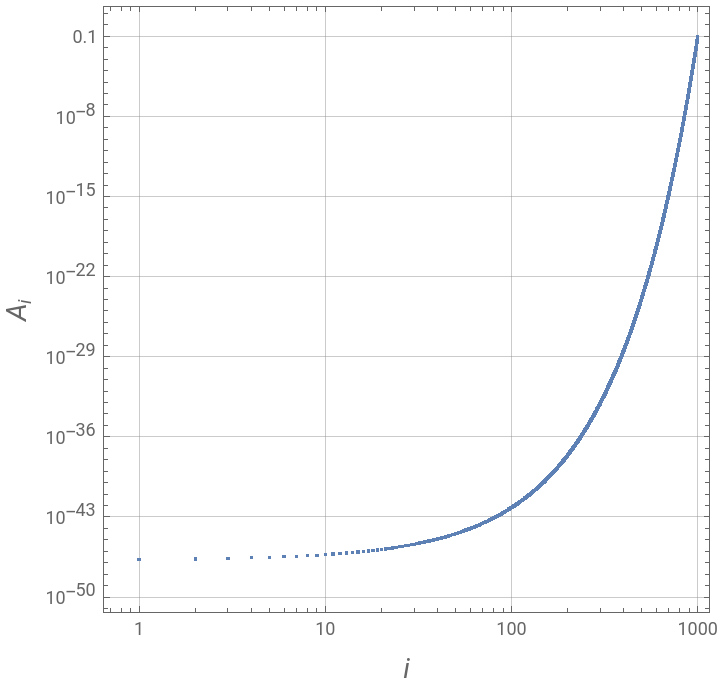
We plot the steady state solutions.
We plot the steady state solutions.
In[]:=
Clear[soleq,eqns];n=1000;A1o=1.;A[0]=0;A[n+1]=0;A[n]=(A1o-Sum[A[j],{j,1,n-1}]);k[0,1]=0;k[1,0]=0;k[n,n+1]=0;k[n+1,n]=0;Table[k[i,(i+1)]=1.,{i,1,n}];Table[k[(i+1),i]=.9,{i,1,n}];
In[]:=
eqns=Table[0k[j-1,j]A[j-1]-(k[j,j-1]+k[j,j+1])A[j]+k[j+1,j]A[j+1],{j,1,n-1}];
In[]:=
soleq=NSolve[eqns,Table[A[j],{j,1,n-1}]];
In[]:=
A[n]=(A1o-Sum[A[j],{j,1,n-1}])/.soleq
Out[]=
{0.1}
In[]:=
Flatten[Table[A[j],{j,1,n}]/.soleq]
Out[]=
In[]:=
ListLogLogPlot[Flatten[Table[A[j],{j,1,n}]/.soleq],Frame->True,GridLines->Automatic,AspectRatio->1,FrameLabel->{Style["i",14,Italic],Style["",14,Italic]}]
A
i
Out[]=
Transient solution for n reactions
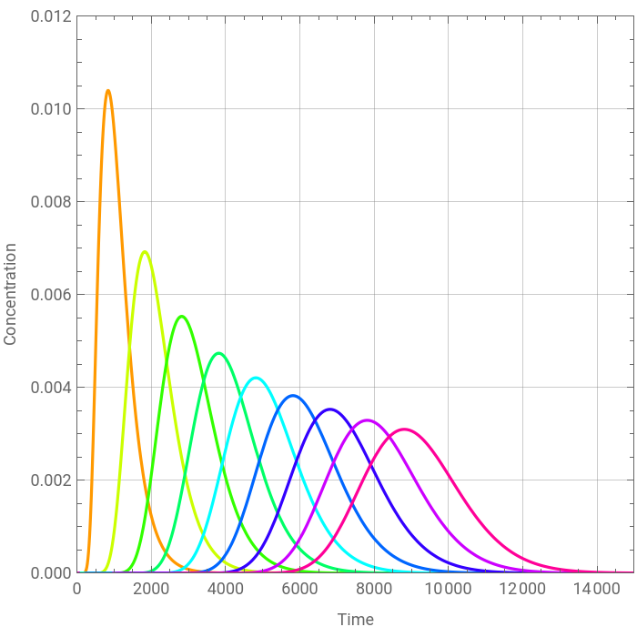
We plot the concentration profile for species:, , , , , , , and .
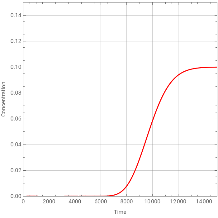
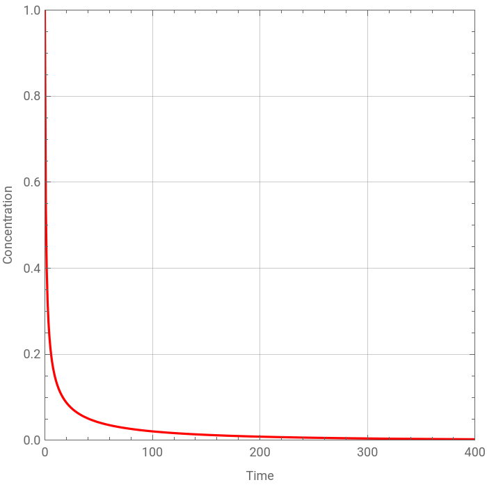
We also plot the concentration profile for, and finally we plot the concentration profile for .
We plot the concentration profile for species:
A
100
A
200
A
300
A
400
A
500
A
600
A
700
A
800
A
900
We also plot the concentration profile for
A
1
A
1000
In[]:=
Clear[soleq,eqns];tf=50000;n=1000;A1o=1.;[t]=0;[t]=0;[t]=A1o-Sum[[t],{j,1,n-1}];k[0,1]=0;k[1,0]=0;k[n,n+1]=0;k[n+1,n]=0;Table[k[i,(i+1)]=1.,{i,1,n}];Table[k[(i+1),i]=.9,{i,1,n}];
A
0
A
n+1
A
n
A
j
In[]:=
eqns[j_]=D[[t],{t,1}]k[j-1,j][t]-(k[j,j-1]+k[j,j+1])[t]+k[j+1,j][t];
A
j
A
j-1
A
j
A
j+1
In[]:=
soleq=NDSolve[Flatten[Table[eqns[j],{j,1,n-1}],[0]==1,Table[[0]0,{j,2,n-1}]],Table[[t],{j,1,n-1}],{t,0,tf}];
A
1
A
j
A
j
In[]:=
Plot[Evaluate[Table[[t],{j,100,n-1,100}]/.soleq],{t,0,tf},FrameTrue,PlotStyleTable[Hue[100j/(n)],{j,1,n}],FrameLabel{"Time","Concentration"},PlotRange{{0,15000},{0,0.012}},Frame->True,GridLines->Automatic,AspectRatio->1,ImageSize->350{1,1}]
A
j
Out[]=
In[]:=
Plot[Evaluate[[t]/.soleq],{t,0,tf},FrameTrue,PlotStyleHue[1/(n)],FrameLabel{"Time","Concentration"},PlotRange{{0,400},{0,1}},PlotPoints900,Frame->True,GridLines->Automatic,AspectRatio->1,ImageSize->350{1,1}]
A
1
Out[]=
In[]:=
Plot[Evaluate[[t]/.soleq],{t,0,tf},FrameTrue,PlotStyleHue[1000/(n)],FrameLabel{"Time","Concentration"},PlotRange{{0,15000},{0,0.15}},Frame->True,GridLines->Automatic,AspectRatio->1,ImageSize->350{1,1}]
A
1000
Out[]=