Three Physics Problems
Three Physics Problems
The following images illustrate situations whose physics are quite similar to one another. The first image shows someone trying to balance an upright baseball bat on an outstretched palm. Earth’s gravitation pulls the bat downward at the center of mass (CM) of the bat, which is above the support point on the palm. The bat “wants” to fall over. If you’ve ever tried to do this, you’ve experienced how difficult it is to do. You must quickly move the base this way and that, trying to “catch” the falling bat and pull it back upright. The slightest imperfection in placement of your palm, or the slightest breeze causes the bat to start falling and you have to chase it, quickly. Circus performers do something similar, balancing upright wands, but they usually put spinning plates on top of the wands. The gyroscopic effects of the spinning plates resist the tipping over of the wand-and-plate combos, making it much easier to keep them upright longer. However, I have seen skilled athletes balance a baseball bat without gyroscopic help. Maybe they’re cheating and there is a gyroscope inside the bat! But I can’t do it with a regulation baseball bat.

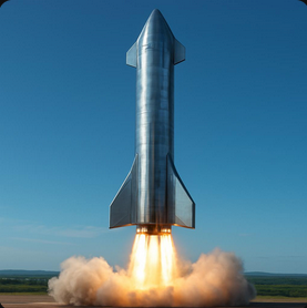
The second image shows a rocket softly landing on its tail. The forces on the rocket include gravitation, pulling downward at the CM, and thrust, pushing upward at the tail. If those forces don’t line up perfectly in the vertical direction, the rocket starts to tip over. The slightest sideways gust of wind, the slightest sideways shift of the CM due to movement of fuel or cargo inside, the slightest imperfection in the angle of the rocket thrust can cause the rocket to tip. The engine exhaust will push the tail very hard, sending the rocket flipping out of control into a disastrous crash. If you’re a fan of rockets, I am sure you have seen this kind of accident—when the rocket tips too far.
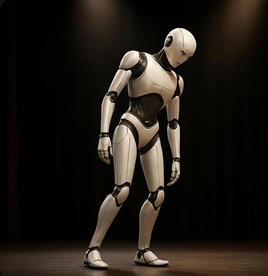
The third image shows a humanoid robot having trouble balancing. Gravitation pulls the robot down at a point above the support on the floor. The robot might not be able to apply enough compensating forces and torques to its feet and ankles quickly enough or to step sideways quickly enough to prevent a fall, again “out of control.”
It’s especially difficult to control an upright robot when it locks its knees. With locked knees, the robot loses a compensating, high-leverage degree of freedom in each knee, plus it takes more time to unlock the knees to squat, bringing the CM closer to the floor and perhaps catching a fall. That’s why robot makers seldom try “underactuated” robots with locked knees: it’s much more difficult to keep them standing up! Instead, we see robots gorilla-walking and doing their tricks and flips with bent knees. That’s cheating!
Another excuse, however, is that it takes a lot of energy to actuate (apply power to) those knees. Humans can’t gorilla walk for more than a few minutes, but humans can balance upright on locked knees for hours on end without conscious effort. With locked knees, the robot situation is closer to the baseball-bat situation and to the rocket situation.
They’re All the Same Problem
They’re All the Same Problem
We can idealize the physics of all three problems the same way: as an upright rod, free to slide on its base on a level, flat plane, with force actuators at the base able to push the base sideways in two dimensions. Think side thrusters for the rocket, or twisting the downwards engines a bit to get a bit (sin θ) of sideways thrust. The robot case is more rich because the feet and knees can apply compensating torques, but we won’t work that case in this notebook.
Remarkably, this problem has an elegant solution when the rod is not tipped too far. It turns out there is a single matrix of numbers, that when multiplied by the current deviation of the system state from upright, yields the forces needed to bring it back upright! This matrix is a Linear Quadratic Regulator (LQR). This matrix has two rows and eight columns. The rows correspond to the two forces we must apply at the base, one in the direction and one in the direction. The columns correspond to the four degrees of freedom (DOFs) and their time derivatives, for a total of eight numbers. The four degrees of freedom are two position variables for the base and two orientation angles to measure the deviation of the rod from upright.
x
y
Let me first show the solution, then show in the Theory Section how to derive the solution from first principles. The animation below is the main contribution of this notebook. To see the animation, there are a few cells to evaluate manually. Those cells can’t be initialization cells for obscure reasons (the notebook failed when I made them initialization cells).
Global Constants
Global Constants
Length of the rod; mass of the rod; mass of the cart; moment of inertia MI of a thin rod about its center of mass; acceleration of Earth’s gravitation and a list of numerical rules. A time limit for numerical integration as a global constant.
d
m
M
g
In[]:=
ClearAll[d,m,M,MI,g,tLim];MI=m;tLim=30;(*seconds*)ClearAll[numRules];numRules={g->9.81,m->1,M->0,d->1};
1
12
2
d
Linearized State Model
Linearized State Model
The temporaries ,, , and the matrices , are derived in the Theory Section below.
C
1
C
2
D
1
D
2
A
l
B
l
In[]:=
ClearAll[C1,D1,Al,C2,D2,Bl,Cl,Dl];With{l=d/2},(*frombasetotheCG*)With{J=4m/3},(*parallel-axistheorem:effectivemomentofinertia*)With{C0=MJ+/3},WithC1=-gC0/.numRules,D1=lgC0/.numRules,C2=JC0/.numRules,D2=-mlC0/.numRules,Al=
;Bl=
;Cl=
;Dl=
;StateSpaceModel[{Al,Bl,Cl,Dl}]
2
l
2
m
2
l
2
m
2
l
2
m
0 | 1 | 0 | 0 | 0 | 0 | 0 | 0 |
0 | 0 | 0 | 0 | C1 | 0 | 0 | 0 |
0 | 0 | 0 | 1 | 0 | 0 | 0 | 0 |
0 | 0 | 0 | 0 | 0 | 0 | C1 | 0 |
0 | 0 | 0 | 0 | 0 | 1 | 0 | 0 |
0 | 0 | 0 | 0 | D1 | 0 | 0 | 0 |
0 | 0 | 0 | 0 | 0 | 0 | 0 | 1 |
0 | 0 | 0 | 0 | 0 | 0 | D1 | 0 |
0 | 0 |
C2 | 0 |
0 | 0 |
0 | C2 |
0 | 0 |
D2 | 0 |
0 | 0 |
0 | D2 |
1 | 0 | 0 | 0 | 0 | 0 | 0 | 0 |
0 | 0 | 1 | 0 | 0 | 0 | 0 | 0 |
0 | 0 | 0 | 0 | 1 | 0 | 0 | 0 |
0 | 0 | 0 | 0 | 0 | 0 | 1 | 0 |
0 | 0 |
0 | 0 |
0 | 0 |
0 | 0 |
Out[]=
0 | 1 | 0 | 0 | 0 | 0 | 0 | 0 | 0 | 0 |
0 | 0 | 0 | 0 | -29.43 | 0 | 0 | 0 | 4 | 0 |
0 | 0 | 0 | 1 | 0 | 0 | 0 | 0 | 0 | 0 |
0 | 0 | 0 | 0 | 0 | 0 | -29.43 | 0 | 0 | 4 |
0 | 0 | 0 | 0 | 0 | 1 | 0 | 0 | 0 | 0 |
0 | 0 | 0 | 0 | 58.86 | 0 | 0 | 0 | -6 | 0 |
0 | 0 | 0 | 0 | 0 | 0 | 0 | 1 | 0 | 0 |
0 | 0 | 0 | 0 | 0 | 0 | 58.86 | 0 | 0 | -6 |
1 | 0 | 0 | 0 | 0 | 0 | 0 | 0 | 0 | 0 |
0 | 0 | 1 | 0 | 0 | 0 | 0 | 0 | 0 | 0 |
0 | 0 | 0 | 0 | 1 | 0 | 0 | 0 | 0 | 0 |
0 | 0 | 0 | 0 | 0 | 0 | 1 | 0 | 0 | 0 |
The meaning of the state-space model is revealed by the standard, first-order state-space form for the linearized equations of motion in terms of the Cartesian Angular Projections α and β . We’ll show two ways to derive these equations in the Theory Section. The prefix “L” stands for “Linear;” the prefix “LL” stands for “Linearized Lagrangian.” These equations describe the physics when α and β are sufficiently small.
In[]:=
ClearAll[LLeqns,LState,LForce];LState={{x[t],x'[t],y[t],y'[t],α[t],α'[t],β[t],β'[t]}};LForce={{fx[t],fy[t]}};(LLeqns=Select[Flatten[MapThread[Equal,{Dt[LState,t],
Al
.LState
+Bl
.LForce
},2]],#=!=True&])//TableFormOut[]//TableForm=
′′ x |
′′ y |
′′ α |
′′ β |
Unit diagonal matrices for the state-residual cost and for the force-application cost suffice for this demonstration. They yield an acceptable LQR, represented by the gains matrix. Tuning Q and R, a topic in controls design, is discussed in a future notebook.
Q
R
In[]:=
ClearAll[stateResidualPenaltyLQ,forcePenaltyLR,gainsL];stateResidualPenaltyLQ=IdentityMatrix[8];forcePenaltyLR=IdentityMatrix[2];(gainsL=(
LQRegulatorGains
[StateSpaceModel
[{Al,Bl,Cl,Dl}],{stateResidualPenaltyLQ,forcePenaltyLR}]//Chop))//MatrixFormOut[]//MatrixForm=
-1. | -2.06318 | 0 | 0 | -25.7842 | -4.50866 | 0 | 0 |
0 | 0 | -1. | -2.06318 | 0 | 0 | -25.7842 | -4.50866 |
We will kick the cart hard in two directions and we can watch it NOT fall over and also recover to equilibrium when we stop kicking in the last half of the animation. Re-evaluate this next cell as often as you like to get new randomized kicking forces:
Highlights are restorations of the standard spherical coordinates θ, ϕ from α and β for display purposes. There is another version of these display routines in the Theory Section for showing the full non-linear solution.
Theory Section
Theory Section
Here, we develop two sets of equations of motion:
1
.Full non-linear Euler-Lagrange equations in standard spherical coordinates, numerically integrated without control forces to show plausible, dangling, swinging motion. These equations are not suitable for linear control because the azimuthal equation diverges at the pole, exactly where we want to stabilize the rod. Nature conspires to make us work harder.
We then linearize both sets of equations about the pole and show that the two linearized sets are identical.
We finally show how to reduce the decoupled equations to the beautiful LQR above via Wolfram’s built-in StateSpaceModel, which performs an independent linearization of the decoupled equations.
Non-linear control of this system is a research topic, active even today. We don’t cover it here.
Full, Non-Linear Equations of Motion
Full, Non-Linear Equations of Motion
Generalized Coordinates
Generalized Coordinates
Potential energy
Potential energy
proportional to the height of the center of mass (CM) of the rod above the plane:
Kinetic Energy
Kinetic Energy
To keep things easy, we’ll build up the velocities by hand, using Wolfram as an assistant.
Angular velocity measured in the inertial frame (by inspection). Remember this expression when we get to linearizing. It’s used here only for assistance in manually constructing the equations:
The CM of the rod in the inertial frame is at position
The following symbolical computation of derivatives ensures the inertial velocities of the CM:
Manually copy inertial velocities into the expression for kinetic energy (manual copying seems the most convenient way to get a function-like, Wolfram expression):
Spot check:
Generalized Forces
Generalized Forces
Generalized Torques
Generalized Torques
Euler-Lagrange Equations
Euler-Lagrange Equations
Numerical Verification of Free Motion
Numerical Verification of Free Motion
Drop the pendulum from not-quite-upright and just off the X-axis. If θ starts off too small, the numerical solution will suffer gimbal lock (Csc[θ] and Cot[θ]) and not act plausibly. However, Wolfram’s numerical integrators have no other difficulty with these substantially non-linear equations. That, itself, is remarkable.
The following animation of free (uncontrolled) motion produces plausible back and forth dangled swinging, verifying the non-linear equations of motion. The animation routines are similar to the ones at the beginning of this notebook, just written directly in terms of co-latitude θ and azimuth ϕ. We did not take the trouble to abstract the common bits of these two sets of animation routines. That’s software engineering, not an objective of this notebook.
Linearizing the Full Non-Linear Equations
Linearizing the Full Non-Linear Equations
A first step to showing that the linearized Euler-Lagrange equations are equal to the linearized decoupled equations (upcoming) is to linearize the Euler-Lagrange equations.
Non-Linear Equations Rewritten and Linearized
Non-Linear Equations Rewritten and Linearized
Atack via a change of variables to Cartesian Angular Projections, α and β, of θ and ϕ onto the plane:
Direct substitution of Equations 3 and 4 into the Euler-Lagrange equations produce unmanageably large expressions. However, we proceed by rewriting the Lagrangian in terms of α and β, linearizing as we go.
First, approximate position and velocity variables from scaling the angular projections by the length of the rod:
Here is linearized kinetic energy TL:
The linearized potential energy is
Our linearized Lagrangian:
We' ll need a Series approximator a couple of times, so let’s abstract it now. Wolfram’s Normal here truncates higher-order terms.
Finally, we can exhibit the four, linearized Euler-Lagrange equations. Again, these are too big to yield ready insight:
As a final step of linearization, we apply the following small-angle approximations
These are small enough to understand intuitively. Once we apply the numerical rules, we see the state-space model from the beginning of this notebook peeking out!
Decoupled Equations
Decoupled Equations
Decoupling differential equations is a standard approach to non-linear problems in physics. I wanted to cross-check the linearized Euler-Lagrange equations via a non-Lagrangian approach. I arrived at these equations by blunt resection of an earlier 3-DOF solution to this problem, plus trial-and-error guided by physical intuition. They’re still non-linear, and a bit more general than the linearized Euler0Lagrange equations, perhaps surviving for larger angles. They can be inspected for intuitive plausibility. We leave it to your inspection and experimentation to validate them. For brevity, they are presented here without discussion. Their utility in this notebook is two-fold: (1) to check that their linearization is identical to the linearized Euler-Lagrange equations, and (2) to demonstrate Wolfram’s ability to linearize them independently via the built-in StateSpaceModel.
Linearized Decoupled Equations
Linearized Decoupled Equations
After applying the following small-angle approximations and a little symbolical massage, these equations are manifestly equal to the linearized Lagrangian equations above.
Here are the numerical linearized decoupled equations, equivalent to all the other expressions of such in this notebook.
Again Linearizing the Decoupled Equations
Again Linearizing the Decoupled Equations
Let’s show that Wolfram’s StateSpaceModel built-in can linearize the decoupled equations independently. This amounts to a round-trip checking of all our math. This time, we get a state-space model we can feed into Wolfram’s LQRegulatorGains to get the beautiful LQR at the beginning of this notebook.
With numerical rules applied, we see exactly the state-space model from the beginning of this notebook.
Finally, we can justify the symbolic constants in the first expression of the state-space form at the beginning of this notebook. Compare these terms to the matrices at the beginning of this notebook and to the two above.
CITE THIS NOTEBOOK
CITE THIS NOTEBOOK
Land a rocket or balance a robot: linear quadratic regulator control of sliding-base inverted rod
by Brian Beckman
Wolfram Community, STAFF PICKS, November 11, 2025
https://community.wolfram.com/groups/-/m/t/3581351
by Brian Beckman
Wolfram Community, STAFF PICKS, November 11, 2025
https://community.wolfram.com/groups/-/m/t/3581351