Exploring Wolfram Quantum Computation Framework
by Subhojit Pal
Indian Institute of Science Education and Research, Bhopal
by Subhojit Pal
Indian Institute of Science Education and Research, Bhopal
Wolfram Quantum Framework Computation Framework performs high-level analytic and numeric computations in Quantum Information Theory, allowing simulation of quantum circuits and quantum algorithms. In this essay, I explore a few quantum algorithms and explore their implementation in the Wolfram Quantum Computation Framework
Installing the paclet
Installing the paclet
Paclet is a library of Mathematica whose purpose to simulate quantum circuits and solve problems of quantum computation and quantum mechanics. Using this library, we can introduce high-level analytic and numerical computations in quantum information theory. Here I have come across quantum operators, quantum states, measurements etc. I have installed this library using the code below. This code will perfectly work on Mathematica V.13 and version 12.3. It will not work on V.12.
In[]:=
PacletUninstall/@PacletFind["Quantum*"];ClearAll["*QuantumFramework*","Wolfram`QuantumFramework`*","Wolfram`QuantumFramework`**`*"];PacletInstall[CloudObject["https://wolfr.am/DevWQCF"],ForceVersionInstall->True]<<Wolfram`QuantumFramework`
Out[]=
PacletObject

Decomposition of some quantum gates
Decomposition of some quantum gates
When working with quantum gates, a very important feature is if and how one can decompose a quantum gate into sequences of such simpler (or universal) gates. In this section, I will explore a few examples and show such decomposition. Of course, at this level, I have done the decomposition manually and only showed the equivalency of results. But a future plan would be doing the decomposition automatically.
For each example in the following, I showed what I plan to test as the heading, then I construct the left and then right side of relationship, and finally I test they are identical.
NOT≡Rx(π).Ph(π/2)
NOT≡(π).Ph(π/2)
R
x
In[]:=
ph[angle_]:=QuantumOperator[{"GlobalPhase",angle}];qc1=QuantumOperator[{"XRotation",π}]@ph;QuantumOperator["NOT"]==qc1
π
2
Out[]=
True
NOT≡Ry(π).Rz(π).Phπ2
NOT≡(π).(π).Ph
R
y
R
z
π
2
In[]:=
Ry[angle_]:=QuantumOperator[{"YRotation",angle}]Rz[angle_]:=QuantumOperator[{"ZRotation",angle}]qc2=Ry[π]@Rz[π]@ph;QuantumOperator["PauliX"]==qc2
π
2
Out[]=
True
NOT≡Rxπ2.Phπ4
NOT
≡R
x
π
2
π
4
In[]:=
Rx[angle_]:=QuantumOperator[{"XRotation",angle}]qc3=Rx@ph;QuantumOperator["RootNOT"]["Matrix"]==ComplexExpand@qc3["Matrix"]
π
2
π
4
Out[]=
True
Note I used ComplexExpand to expand
ϕ
NOT≡Rz-π2.Ryπ2.Rzπ2.Phπ4
NOT
≡R
z
-π
2
R
y
π
2
R
z
π
2
π
4
In[]:=
qc4=Rz@Ry@Rz@ph;QuantumOperator["RootNOT"]["Matrix"]==ComplexExpand@qc4["Matrix"]
-π
2
π
2
π
2
π
4
Out[]=
True
H≡Rx(π).Ryπ2.Phπ2
H≡(π)..Ph
R
x
R
y
π
2
π
2
In[]:=
qc5=Rx[π]@Ry@ph;QuantumOperator["H"]==qc5
π
2
π
2
Out[]=
True
H≡Ryπ2.Rz(π).Phπ2
H≡.(π).Ph
R
y
π
2
R
z
π
2
In[]:=
qc6=Ry@Rz[π]@ph;QuantumOperator["H"]==qc6
π
2
π
2
Out[]=
True
Rx(θ)≡Rz-π2.Ry(θ).Rzπ2
R
x
R
z
-π
2
R
y
R
z
π
2
In[]:=
Rx[theta_]:=QuantumOperator[{"XRotation",theta}]qc7[theta_]:=Rz@Ry[theta]@Rz;Rx[θ]["Matrix"]==Map[FullSimplify[#,θ∈Reals]&,ComplexExpand@qc7[θ]["Matrix"],{2}]
-π
2
π
2
Out[]=
True
Note I used ComplexExpand to expand and also simplify it, to test equality.
ϕ
Rx(θ)≡Ryπ2.Rz(θ).Ry-π2
R
x
R
y
π
2
R
z
R
y
-π
2
In[]:=
Rz[theta_]:=QuantumOperator[{"ZRotation",theta}]qc8[theta_]:=Ry@Rz[theta]@Ry;Rx[θ]["Matrix"]==Map[FullSimplify[#,θ∈Reals]&,ComplexExpand@qc8[θ]["Matrix"],{2}]
π
2
-π
2
Out[]=
True
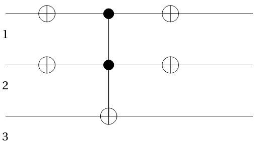
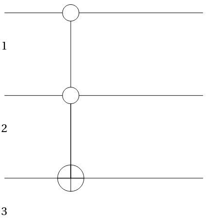
Controlled-0 gate with two control qubits
Controlled-0 gate with two control qubits
In[]:=
qc1=QuantumCircuitOperator[{QuantumOperator["NOT"],QuantumOperator["NOT",{2}],QuantumOperator["Toffoli"],QuantumOperator["NOT"],QuantumOperator["NOT",{2}]}];qc1["Diagram"]
Out[]=
In[]:=
u=QuantumOperator["NOT",{3}];qc2=QuantumCircuitOperator[{QuantumOperator[{"Controlled0",u,{1,2}}]}];qc2["Diagram"]
Out[]=
SWAP combined with an arbitrary controlled-U
SWAP combined with an arbitrary controlled-U
Controlled0-U
Controlled0-U
CNOT and modified CSIGN
CNOT and modified CSIGN
Decomposition of CNOT
Decomposition of CNOT
Superdense coding
Superdense coding
Here in this protocol we will send two classical bit of information by one qubit. First we have to create a Bell pair by “H” and “CNOT” gate which will be shared by two parties as Alice and Bob. Now Alice encodes her messages as “00”, “01”, “10” and “11”. And she performs some quantum operation according to the encoded information like she does I for “00” , “X” for “01”, “Z” for “10” and “ZX” for “11”. Then she sends this to Bob. Bod has done first “CNOT” operation and then “H” to get the actual information send by Alice. Here We have used four qubits two for Alice and two for Bob. At the third qubit “H” and “CNOT” create Bell pair which will depend on bit structure of qubit 3 and 4. And then done some operations(I, X, Z, ZX) and the performs “ CNOT” and “H”. And then measure the qubit 3 and and 4.
Here the state function is initial state and the list {x,y} is the bit what Alice wants to send to Bob. And Tuples create the four states as 00, 01, 10 and 11 and probability plot shows the probability of each state in different cases separately with 100% probability.
Keywords
Keywords
◼
Quantum Computation
◼
Superdense Coding
Acknowledgment
Acknowledgment
Firstly and foremost, I would like to thank Mads Bahrami for his unequivocal help without whom this essay could not have been completed. His positive and nurturing attitude made the school very fun and possible to cope even with difficult C-19 circumstances. I also express my gratitude to Rahul Sharma, TA, for helping me resolve bugs and explain me things through the duration of this winter experience. My sincere regards to Tuseeta Banerjee for being understanding, Mads and the entire Organising Team for taking us on this educational journey. Lastly, I will not forget my Physics professor, Dr Arnab Rudra, who had told me about this amazing school.
References
References