We introduce a computational framework for exhaustive generation of biased cellular-automaton aggregation systems and discuss its influence on structural density. We present a modification of the AggregationSystem resource function which, for any given rule and initial grid, enumerates every possible single-cell update for the generations of a multiway state-space. We then identify terminal states (end-state nodes with no outgoing transitions) and overlay path-highlighting from the origin to each terminal via vertex- and edge-coloring to reveal emergent convergence patterns. These subgraphs are then analyzed via methodology from spectral graph theory, revealing patterns in connectivity, entropy, and other properties of multiway systems. Such analyses of discrete dynamical systems can be adapted to model a variety of physical and networked processes.
Introduction
Introduction
Cellular Automata (CA) models are representations of evolving systems on a state space where complex structures may emerge from simple local rules. This paper defines the state space as a grid where an initial tile, or cell, detects the states of its adjacent cells, or “neighbors,” and updates itself. These rules can lead to various emergent behavior over large numbers of these updates, or “iterations.”
In[]:=
GraphicsRow[Table[ArrayPlot[CellularAutomaton[x,{{1},0},75]],{x,{30,150,182}}],ImageSize->Full]
Sample cellular automata of rules 30, 150, and 182 over 75 iterations.
Out[]=

Aggregation systems are a type of cellular automata such that the set of defined rules does not include the removal of previously occupied cells, leading to structures where new cells get added around a cell following a ruleset related to its neighbors. Over time, these typically aggregate into large clusters of cells.
In[]:=
StyleMapArrayPlotCenterArray[#,(Max[Dimensions[#]]+2){1,1}],Mesh->False,MeshStyle["MeshStyle",1],ImageSize->80&,SeedRandom[9999];[Range[4]]Range[4],[2,4],{{0,0}},9,LineSpacing->{1,10}
Row display of every single iteration from 1 through 9 of the Eden cellular automaton model.
In[]:=
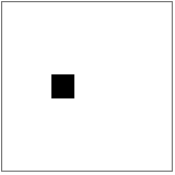





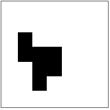
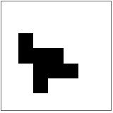
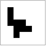
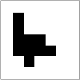
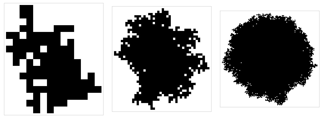
Shown above is the complexity-minimized “Eden model,” where the initial state of the system is one black cell, and for each iteration, a new black cell is randomly added on an unoccupied square vertically or horizontally adjacent to an existing cell. Below is the same system after one hundred, one thousand, and ten thousand iterations. The random choice of candidate cells that are placed in each iteration is governed by a random seed via the SeedRandom[] function, which acts upon the RandomAggregation resource function.
In[]:=
showcaseAgg[itr_]:=ArrayPlot[Range[4]]SeedRandom[9999];LastRange[4],[2,4],{{0,0}},itr,FrameStyle->["FrameStyle"]GraphicsRow[{showcaseAgg[100],showcaseAgg[1000],showcaseAgg[10000]}]
Row display of the Eden cellular automaton model after 100, 1,000, and 10,000 iterations.
Out[]=
We can add further restrictions to the generation rules of an aggregation system. At the pre-generation (determination candidate cells) step, we can specify the domain in which the rules may apply. The Von Neumann or 4-cell neighborhood considers only vertically and horizontally adjacent cells, both during pre-generation and generation (placement of cells) stages. We can also be specify the number(s) of neighbors of a cell required for that cell to be eligible for growth. This is referred to as a “totalistically constrained growth,” some examples of which are shown below.
In[]:=
Module{rules,res},rules=Subsets[Range[5]];res=LastSeedRandom[9999];#,[2,4],Position[CrossMatrix[{1,1}],1]-2,10&/@rules;res=Map[If[FailureQ[#],#["Data"],#]&,res];res=Map[CenterArray[#,{11,11}]]&,[{}][res];MapThreadLabeledArrayPlot#1,Mesh->True,MeshStyle["MeshStyle",0],ImageSize->60,Text@Row[{Style["4: ",10],Style[#2,12]}],Spacings{0,0}&,{res,rules}
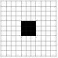
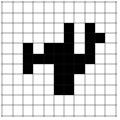
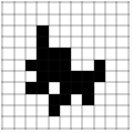
Row display of cellular automata evolutions under all rules 𝑟 ∈ 𝑅 ⊆ Range[5], with a Von Neumann neighborhood, after 20 iterations. 4 denotes the 4-neighbor rules and integers within the curly brackets denote the number(s) of neighbors serving as growth conditions. As an example, “4: {1,2}” suggests a 4-neighbor rule where an unoccupied cell needs to have exactly one or two neighbors to be eligible for growth. These rules can be specified via the $NeighborhoodData resource function.
Out[]=
,
,
,
,
,
,
,
,
,
,
,
,
,
,
,
,
,
,
,
,
,
,
,
,
,
,
,
,
,
,
,
4: {} |
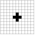
4: {1} |
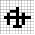
4: {2} |
4: {3} |
4: {4} |
4: {5} |
4: {1,2} |
4: {1,3} |
4: {1,4} |
4: {1,5} |
4: {2,3} |
4: {2,4} |
4: {2,5} |
4: {3,4} |
4: {3,5} |
4: {4,5} |
4: {1,2,3} |

4: {1,2,4} |
4: {1,2,5} |
4: {1,3,4} |

4: {1,3,5} |
4: {1,4,5} |
4: {2,3,4} |
4: {2,3,5} |
4: {2,4,5} |
4: {3,4,5} |
4: {1,2,3,4} |

4: {1,2,3,5} |
4: {1,2,4,5} |
4: {1,3,4,5} |
4: {2,3,4,5} |
4: {1,2,3,4,5} |
One should notice an emerging pattern in the final states of the systems after 20 iterations: identical “terminal states” where the growth rule does not permit any more placing of cells. When such structures are limited by an n number of neighbors (take the example of {2} in this case, rules that consist of only greater integers n + m will also take the same form of terminal states. The same pattern appears with rules that include only {3} and combinations of it with greater integers, where the same terminal state is shown.
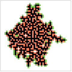
Constraints on the growth of aggregation systems can be conveniently visualized via the coloring of cells. We define:
as cells that are currently part of the system, or “alive” cells,
as cells that are not yet part of the system or connected to the main system cluster,
as cells that are immediate candidates (in other words, they belong in the pool of possible cells that will turn black in the next iteration of the system) that may be picked by random chance
are cells that may potentially become green cells in a future iteration since they do not yet reach the required number of neighbors
as cells that can no longer become part of the system.
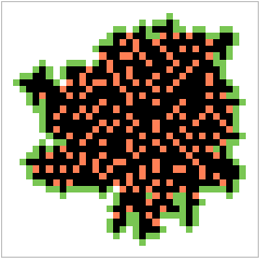
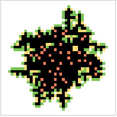
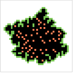
In the cases of some rules, orange tiles contribute to the generation of two of the most prominent features of a multiway aggregation system: holes and terminal states. In the following sections of this paper, we discuss an essential property that emerges in correspondence with porous growth—density.

In the cases of some rules, orange tiles contribute to the generation of two of the most prominent features of a multiway aggregation system: holes and terminal states. In the following sections of this paper, we discuss an essential property that emerges in correspondence with porous growth—density.
In[]:=
GridPartitionLabeled[#]LastSeedRandom[9999];#,[2,4],Position[CrossMatrix[{1,1}],1]-2,500,FrameStyle->["FrameStyle"],ImageSize->120,Mesh->False,"Boundary"->True,Padding->1,Text@Row[{Style["4: ",10],Style[#,12]}],Spacings->{0,0}&/@Select[Subsets[Range[3]],MemberQ[1]],4,Spacings->{0,0}
Row display of rule-correspondence boundary-colored cellular automata evolutions under all rules 𝑟 ∈ 𝑅 ⊆ Range[3], with a Von Neumann neighborhood, after 500 iterations.
Out[]=
|
|
|
|
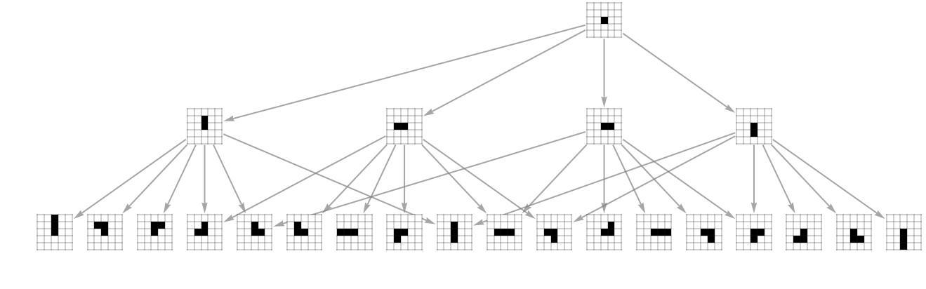
Multiway systems model every possible path of evolution for a given system, where one state can lead to multiple unique ones. In the case of aggregation systems, the effect of the defined rules on every iteration is shown as a branching vertex on a path, from one previous state to another newer one. Expanding on the previous discussion, the Eden model can be displayed via a multiway system :
In[]:=
Graph[Range[4]]Range[4],[2,4],{{0,0}},2,"Boundary"->False,"Centering"->False,Padding->0,AspectRatio->14,VertexSize->1.5,GraphLayout->"LayeredDigraphEmbedding"
Multiway system of all possible evolution states of the Eden cellular automaton model after after 2 iterations.
Out[]=
Some of the states shown in the multiway system are identical and vary only due to trivial transformations such as translation, reflection, or rotation. These groups can be eliminated via canonicalization. Despite this elimination, after only a few iterations, the multiway system becomes extremely complex to the point where it is difficult for any kind of pattern to be analyzed, although varying the forms of graph embedding may aid in the visualization.
In[]:=
GraphRange[4],[2,4],{{0,0}},7,"Canonicalize"->True,EdgeStyle->Gray,AspectRatio->13,VertexSize->.5,GraphLayout->"LayeredDigraphEmbedding"
Multiway systems of all possible evolution states of the Eden cellular automaton model after after 7 iterations via LayeredDigraphEmbedding, RadialEmbedding, and ElectricalEmbedding, respectively.
In a multiway system, terminal states are vertices with no outgoing edges. Graph theory proves quintessential in modeling all sorts of systems, from dynamical to logical. One especially useful tool from the field is the spectral theory of graphs—the study of matrices and eigenvalues of various properties of graphs. In later sections of this paper, we employ methods from spectral graph theory to investigate fragments of multiway systems that lead to terminal states in terms of their connectivity, stochasticity, and more.
Quantifying Density in Discrete Aggregation Systems
Quantifying Density in Discrete Aggregation Systems
Unconditioned Aggregation System and Boundary Function
Unconditioned Aggregation System and Boundary Function
aggregationSystem implements a self-contained mechanism for simulating discrete growth on a two-dimensional cellular grid. It takes in a cellular automaton rule and an initial growth site. In accordance with the rule, a set of candidate cells is determined, and a cell is randomly chosen from the candidate set; the newly occupied cell is then committed to the state, and the process repeats. By combining deterministic neighborhood rules with probabilistic site selection, the function generates a single representative realization of an aggregation trajectory until either the requested number of iterations or list of growth event counts is exhausted. The final matrix returned therefore shows the emergent structure dependent on the random seed and rule.
An unpad function to remove all-blank outer layers from a padded array by identifying slices where every element is zero and excising those margins to maintain minimal bounds. aggregationSystem for iterative application of a specified cellular automaton rule to an expanding array, selecting a random nonzero-growth position, updating that cell, and halts when no further growth sites remain or the prescribed number of iterations is reached.
We define a boundary limit as of growth as a two-dimensional quadrilateral grid where there initially exists a starting cell or "nucleation site" of an aggregation system. Said cell then sequentially evolves into an emergent structure of occupied cells whose density is formally calculated as the ratio of occupied cells over the total area, providing a metric for comparative analysis of discrete aggregation behaviors across varied conditions and parameters. The function initially takes in any matrix, its growth rule, a bound size, and optionally a random seed. Utilizing a configurable aggregation rule that permits cell occupation based on specified neighbor conditions, the function iteratively applies this rule until a the predetermined bound of growth in any of the cardinal directions is satisfied.
At each iterative step, the function evaluates the current dimensions of the aggregation matrix, specifically checking if the growth boundary has reached a defined spatial limit. Upon reaching this threshold, the function terminates, producing an aggregated structure visualized through an array plot.
At each iterative step, the function evaluates the current dimensions of the aggregation matrix, specifically checking if the growth boundary has reached a defined spatial limit. Upon reaching this threshold, the function terminates, producing an aggregated structure visualized through an array plot.
boundedAggregationModule initializes a seeded aggregation system on a 3×3 nucleation grid, iteratively grows it until the occupied boundary reaches a specified limit and at least one border cell is occupied, then displays the final configuration along with counts of black/white cells and its density.
Randomness in Bounded Unconditioned Aggregation
Randomness in Bounded Unconditioned Aggregation
The plot below shows how the density (𝜌) of a discrete aggregation structure changes as its boundary limit (ℓ) increases. It computes and plots density curves across boundary limits from 1 to 20 for twenty seeds (seeds number 1 through 20). The resulting plot clearly illustrates both the general upward trend showing that structures typically become denser as they' re allowed more space to grow.
The variability introduced by randomness is represented by different colored curves corresponding to each seed . Despite a noticeable initial trend, the average values of these seeds converge toward a single value, showing an unpredictability and lack of long - term density trend .
Weighting and Corresponding Biased Growth
Weighting and Corresponding Biased Growth
Neighbor Density-Weighted Aggregation
Neighbor Density-Weighted Aggregation
We also define functions for aggregation system CA generation such that a bias is implemented via a “weighting” rule in accordance to the number of neighbors an empty candidate cell has. The integer values of the number of neighbors for a given candidate cell is mapped onto the weight property of the RandomChoice function. For instance, an unoccupied cell with three neighbors will be three times more likely to be chosen for placement when compared to another with one neighbor.
modAggregationSystem simulates a biased stochastic growth process where, at each iteration, a cell is chosen from possible growth sites with probability weighted by local neighbor density, leading to preferential aggregation in denser regions.
The 6x3 plot below shows comparisons between unbiased and linearly biased generation of aggregation systems. The three left columns are unbiased while the three right are linearly biased. Columns one and four, two and five, and three and six share the same seed, while rows one, two, and three shows the boundary sizes 10, 20, and 30 cells, respectively.
A function is defined to provide an interpretive visualization of local spatial density in a binary cellular matrix by computing and displaying the 8 connected neighbor count for each cell. The input matrix is first binarized to distinguish occupied (1) from unoccupied (0) cells, after which a list convolution with a standard Moore neighborhood kernel is applied to produce a neighborCounts map. This map offers a measure of local structural density. The matrix and density map are vertically reversed for visualization fix.
visualizeWithWeights overlays local neighbor density values on a binary aggregation matrix by computing an 8-neighbor count at each cell, reversing the grid for correct display alignment, and annotating non-occupied cells with bold labels indicating their weighted influence in growth atop an ArrayPlot of the current aggregation system state.
We may also represent this neighbor-intensity for each empty cell as different shades of the grayscale.
In accordance with the neighbor weight array plot, we can also calculate the probability for each candidate cell for being placed in the next iteration of the system and display it in their respective cells.
visualizePlacementProbabilities displays a binary aggregation matrix overlaid with the exact probability of each candidate cell being selected for growth, based on normalized neighbor weights from an 8-connected convolution kernel. It identifies valid growth sites, computes their local-density-based probabilities, and annotates each with a bold text label on the reversed matrix layout, enabling visual inspection of stochastic placement likelihoods.
Multiway Graphs of Aggregation Systems
Multiway Graphs of Aggregation Systems
Terminal State Candidate Conditions
Terminal State Candidate Conditions
The resource function NestWhileGraph[] with different (mainly the layered digraph) embeddings may be used to generate multiway systems showing the possible evolutions of an aggregation system. Consider an elementary non-aggregation system example where three functions are applied to a matrix for each iteration is shown below.
Three simple addition functions on a matrix for NestWhileGraph iteration.
Vertices that are possible candidates for terminal states may be identified by a highlighting function showing all vertices in a graph that only has edges directed into it. Recall that this list of vertices may include, in addition to actual terminal states, non-terminal states that are limited by the iteration number rather than ability to continue growing.
Identify terminal vertices and highlight them in red.
Subgraph Separation Function and Terminal Configuration
Subgraph Separation Function and Terminal Configuration
We also define functions that take all possible paths between two vertices and highlights
highlightSubgraph takes in a graph and two of its vertices then highlights every possible path between the two with directed edges for the use case of multiway systems.
These paths are their own separate graphs, or rather, fragments of the full multiway system. We extract these subgraphs out for comparison and further analysis in the following section. Graph theoretic properties of these subgraphs not only provide us with a more complete picture of the multiway system as a whole, but also more precise information on its terminal states.
separateSubgraph works in relation with the highlightSubgraph function, where the highlighted part of a larger graph with the extracted vertices and edges data are created into a separate subgraph.
These functions are critical for analysis of various properties of directed acyclic graphs—graphs whose edge “flow forward” relative to time—like our multiway systems. While some graph theoretic metrics give us insights on the overall structure of large multiway systems, comparative analyses between certain subgraphs can also give us a more detailed picture of the systems’ properties. We take a known terminal state found at the ninth iteration of the 8-neighbor rule {2} aggregation multiway system. Below is the multiway graph of this aggregation system after 9 steps.
Examining a part of the multiway system more closely, we see that there exists a state at the end of the highlighted graph path that restricts any further growth. As the rules require exactly two neighbors for another cell to be placed and there is no cell that fulfills this requirement, the set of candidate cells is empty, and this branch of the multiway system is terminated, hence a terminal state.
Extracting out the subgraph of all possible paths leading to the terminal state gives us:
This terminal state is quite rare in our multiway system. Taking the ratio of all possible paths in the extracted subgraph to that of the multiway system yields a probability of ~1.5% of reaching this state. This means that there is quite a weak notion of confluence seen from the lack of convergence towards a certain state and thereby the high likelihood of more edges being directed out of each vertex making the multiway system larger for each iteration.
Automorphisms and Spectral Graph Theoretic Analysis
Automorphisms and Spectral Graph Theoretic Analysis
Structural and Spectral Characteristics of Terminal States
Structural and Spectral Characteristics of Terminal States
Computes the algebraic connectivity of a graph by calculating the second-smallest eigenvalue of its normalized Laplacian matrix.
High 𝐻 indicates a rich and complex mix of frequencies (structural irregularity), while low 𝐻 reflects a more uniform or symmetric spectrum. Applying this to each terminal-state subgraph lets us quantify and compare their local structural complexity in a single, comparable scalar. Having identified these terminal states and their structural properties, we now turn toward a deeper graph-theoretic exploration of the entire aggregation system.
Computes the spectral entropy of a graph by applying the Shannon entropy formula to the normalized absolute eigenvalues of its adjacency matrix.
Below are multiway graphs of aggregation systems of rules {1}, {2}, {3} (first row), {1,2}, {1,3}, {2,3}, {1,2,3} (second row) after three iterations as well as their calculated values of algebraic connectivity and spectral entropy.
Automorphisms and Symmetry
Automorphisms and Symmetry
Automorphism analysis reveals structural symmetries in multiway aggregation graphs, identifying when distinct growth histories converge to indistinguishable configurations. This is perfect for our system, as many biased cellular updates lead to superficially distinct but structurally equivalent outcomes—automorphisms let us collapse these redundancies and expose the true causal skeleton of the system. We continue the discussion on the rule {2} aggregation system at ten iterations, where a terminal state is identified at the ninth iteration. We first identify all possible terminal states in the multiway system.
Examining every path toward all the terminal candidates, we find that vertex 316 occurs at the ninth iteration, proving to be our previously known terminal state. This section of the terminal identification process demonstrates the possibility to “work backwards,” or in other words, post-generation, toward any terminal state in a multiway system.
In this case, utilizing the GraphAutomorphismGroup[] function returns no nontrivial permutation groups that could aid the elimination or canonicalization of terminal state paths. The process of identifying terminal cells is done through taking a list of all candidate terminal cells, creating subgraphs of all possible paths between them and the original state, then compare the lengths of the paths. If there exists a terminal state for at iteration n, then its path length will be one shorter than all other candidates at iteration n + 1. Unfortunately, a limitation of computation power restricts further investigation on the automorphisms of terminal state subgraphs from multiway aggregation systems.
Conclusions
Conclusions
This project demonstrated how different bias mechanisms: unbiased, linear, and exponential, affect the density evolution of aggregation systems over time. These results highlight the sensitivity of the system to local attachment preferences and suggests that tunable bias could serve as a controllable parameter for steering emergent material properties in simulated or real-world self-assembly processes.
In addition to structural analysis, this work demonstrated how multiway systems can be used to model the dynamics of aggregation processes, revealing the rich combinatorial and geometric structures that emerge from simple local rules. By applying spectral graph theoretic methods such as algebraic connectivity and spectral entropy, we were able to quantify global cohesion and local complexity across different rule sets and growth regimes. Despite computational challenges at larger scales, the results highlight how multiway networks serve as a powerful framework for understanding constrained versus stochastic growth. These methods pave the way for future investigations into symmetry, topological invariants, and physical analogs of crystallization and disorder in discrete systems.
In addition to structural analysis, this work demonstrated how multiway systems can be used to model the dynamics of aggregation processes, revealing the rich combinatorial and geometric structures that emerge from simple local rules. By applying spectral graph theoretic methods such as algebraic connectivity and spectral entropy, we were able to quantify global cohesion and local complexity across different rule sets and growth regimes. Despite computational challenges at larger scales, the results highlight how multiway networks serve as a powerful framework for understanding constrained versus stochastic growth. These methods pave the way for future investigations into symmetry, topological invariants, and physical analogs of crystallization and disorder in discrete systems.
Future Directions
Future Directions
Overcoming computational constraints, specifically as the number of iterations or the complexity of rule sets increased, would drastically accelerate the range and depth of analyses that can be performed on multiway graphs of aggregation systems. Technical future outlooks include optimizing memory-efficient representations, incorporating probabilistic sampling of paths or terminals, and exploring richer topological and categorical invariants beyond basic spectral descriptors.
Looking ahead, the same approaches and methods can be scaled to larger lattices, higher dimensions, or more intricate rule sets, making it a versatile platform for the study of diverse discrete dynamical systems. Highlighted in Stephen Wolfram’s article, there are much more that can be done even merely in the context of mathematical theory. Take for example the geometric manipulation of cell and state space shapes.
One could also create aggregation systems in three-dimensional space. There has been works that explore properties such as density and cube connectivity in three-dimensional aggregating cellular automata.
Aggregation systems, given sufficiently complex sets of generation rules, boundaries, dimension limitations, or iterations, can be also serve as potent utilities for modeling a wide range of chemical and physical systems, from transport phenomena to subatomic particle movements.
Acknowledgements
Acknowledgements
This work would not have been possible without the guidance and insight of my mentor Adam Millar through every stage of the project. I am grateful to the other mentors and teaching assistants of the Wolfram Summer Research Program who aided me during this project, including, in no particular order; Lyman Hurd, Jason Sonnenberg, Anoushka Munchhal, and William Choi-Kim, all of whom provided kind assistance and thoughtful discussions throughout the process. I sincerely thank the program directors for providing all research scholars with this invaluable opportunity. Finally, I extend my appreciation Stephen Wolfram whose foundational work and vision made this project possible.
References
References
◼
Stephen Wolfram (2023), “Aggregation and Tiling as Multicomputational Processes,” Stephen Wolfram Writings. https://writings.stephenwolfram.com/2023/11/aggregation-and-tiling-as-multicomputational-processes
◼
Yufan Wang (2024), “On chaos in aggregation systems,” Wolfram Community. https://community.wolfram.com/groups/-/m/t/3215676
◼
Daniel Spielman (2025), “Spectral and Algebraic Graph Theory,” Department of Computer Science, Yale University. https://www.sciencedirect.com/topics/computer-science/spectral-entropy
◼
Fan R.K. Chung (1997), “Spectral Graph Theory,” American Mathematical Society. https://mathweb.ucsd.edu/~fan/research/revised.html
◼
Wolfram Education Programs (2024), “Cellular automata generation of 3D printer infill,” Wolfram Community. https://community.wolfram.com/groups/-/m/t/3379925
CITE THIS NOTEBOOK
CITE THIS NOTEBOOK
On the density and multiway spectral theory of aggregation systems
by Thantham Jittham
Wolfram Community, STAFF PICKS, July 11, 2025
https://community.wolfram.com/groups/-/m/t/3503509
by Thantham Jittham
Wolfram Community, STAFF PICKS, July 11, 2025
https://community.wolfram.com/groups/-/m/t/3503509