Single qubit gates with pulses
Single qubit gates with pulses
PacletInstall["Wolfram/QuantumFramework"];<<Wolfram`QuantumFramework`<<Wolfram`QuantumFramework`SecondQuantization`
Form of the trapping potential, where the ,,ϕ can be tuned to effectively trap the ion. Saddle shaped potentials when rotated can realize confinement of ions
u
i
v
i

Out[]=

In[]:=
ionBasis=QuantumBasis[{"g","e"}];
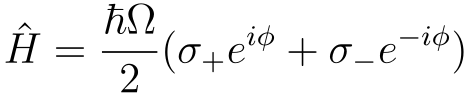
After simplifications and approximations an ion resonant to laser can be described by the Hamiltonian:where Ω is the Rabi frequency and ϕ is an initial displacement of light
In[]:=
H=QuantumOperatorQuantumOperator["JZ+",ionBasis]+QuantumOperator["JZ-",ionBasis],"Parameters"->ϕ
Ω
2
ϕ
-ϕ
Out[]=
QuantumOperator


Evolutions of |g〉 and |e〉 states:
In[]:=
evolution=QuantumEvolve[H,None,t]//FullSimplify;
In[]:=
evolution@QuantumState["0",ionBasis]//ComplexExpand//FullSimplify//TraditionalForm
Out[]//TraditionalForm=
cos|g〉+sin(sin(ϕ)-cos(ϕ))|e〉
tΩ
2
tΩ
2
In[]:=
evolution@QuantumState["1",ionBasis]//ComplexExpand//FullSimplify//TraditionalForm
Out[]//TraditionalForm=
sin(-sin(ϕ)-cos(ϕ))|g〉+cos|e〉
tΩ
2
tΩ
2
Getting the Hadamard gate with a sequence of 5 pulses (with extra global phase of ):
In[]:=
hadamard5pulses=evolution0,@evolutionπ2,@evolution0,@evolutionπ2,@evolution0,;
π
2Ω
π
2Ω
π
2Ω
π
2Ω
-π
2Ω
In[]:=
hadamard5pulses==QuantumOperator["H",ionBasis]
Out[]=
True
Getting the T gate with a sequence of 3 pulses (with extra global phase of ):
π/8
In[]:=
T3pulses=evolution0,@evolutionπ2,@evolution0,;
π/8
π
2Ω
π
4Ω
-π
2Ω
In[]:=
QuantumOperator["T",ionBasis]==T3pulses
Out[]=
True
Just with H and T gates any operator on group SU(2) can be approximated with arbitrary precision, implementing any single qubit gate
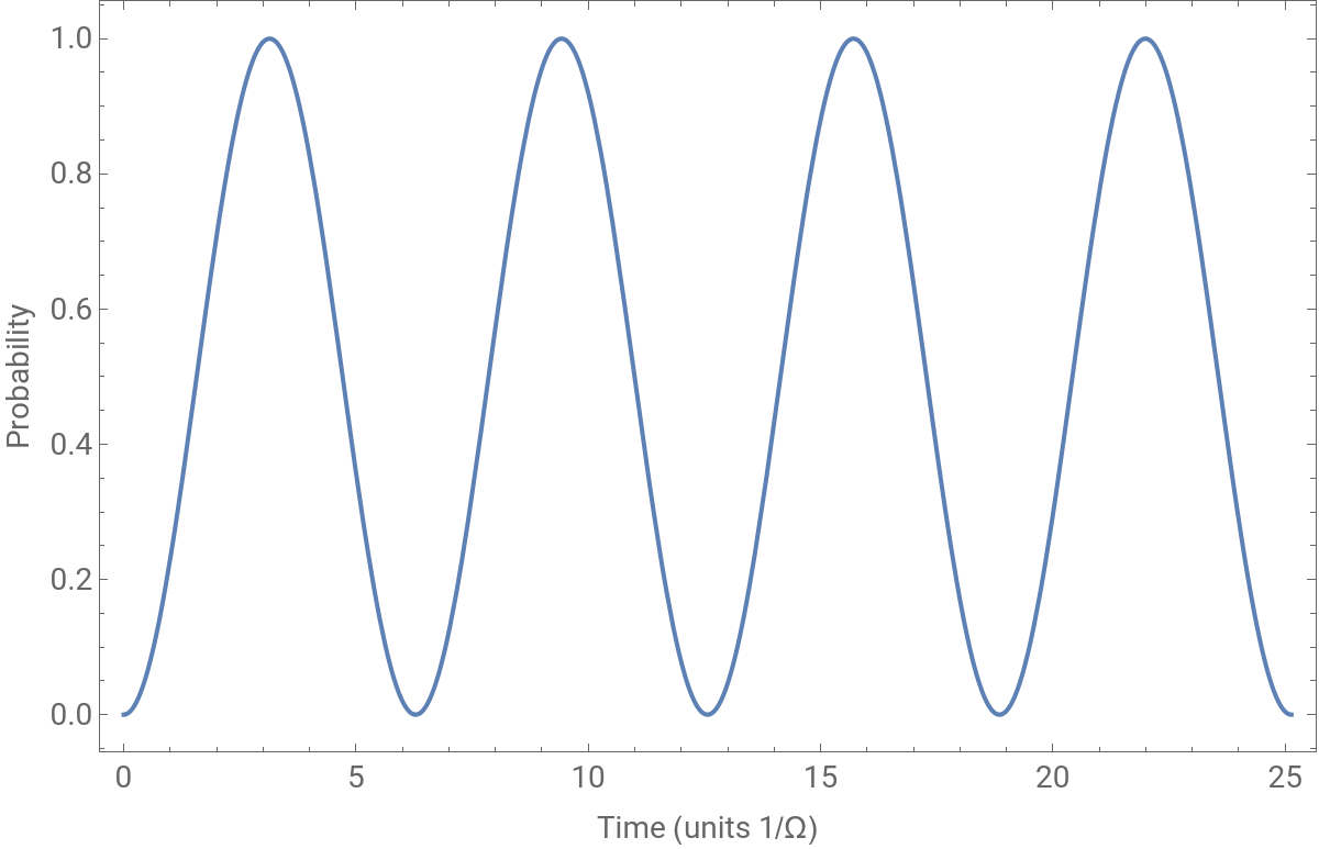
Plotting probability of finding the ion in excited state with ϕ = 0, behavior known as Rabi oscillations:
In[]:=
Plot[Evaluate@evolution[0,t/Ω][]["Probability"][[2]],{t,0,8π},Frame->True,FrameLabel->{"Time (units 1/Ω)","Probability"},LabelStyle->14,ImageSize->600]
Out[]=
The evolution operator dependent on ϕ, t and Ω corresponds to a general rotation with parameters :
tΩ,ϕ-π/2,π/2-ϕ
In[]:=
MatrixForm[m1=evolution[ϕ,t]["Matrix"]//ExpToTrig]
Out[]//MatrixForm=
Cos tΩ 2 | -Cos[ϕ]Sin tΩ 2 tΩ 2 |
-Cos[ϕ]Sin tΩ 2 tΩ 2 | Cos tΩ 2 |
In[]:=
MatrixForm[m2=QuantumOperator["U3"[tΩ,ϕ-π/2,π/2-ϕ]]["Matrix"]//ExpToTrig]
Out[]//MatrixForm=
Cos tΩ 2 | -Cos[ϕ]Sin tΩ 2 tΩ 2 |
-Cos[ϕ]Sin tΩ 2 tΩ 2 | Cos tΩ 2 |
In[]:=
m1-m2//Normal
Out[]=
{{0,0},{0,0}}
Ion chain phonon motional states
Ion chain phonon motional states
The whole ion chain behaves as a QHO with phonon states |n〉 with fundamental frequency ω under Lamb-Dicke regime:
Phonon annihilation operator:
In[]:=
a:=AnnihilationOperator[10];
Define a basis of two ions and truncated phonon space of 10:
In[]:=
twoSpinchain=QuantumBasis[{ionBasis,ionBasis,QuantumBasis[10]}];
In[]:=
QuantumState["000",twoSpinchain]
Out[]=
|gg0〉
Depending on the frequency of the laser we can get different transitions:
If=ω+Δ induces blue sideband transitions
If=Δ-ω induces red sideband transitions
If=Δ is just a carrier transition
If
ω
b
If
ω
r
If
ω
c
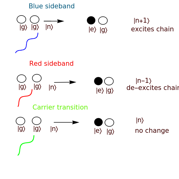
If pulse is on the first ion:
In[]:=
bluesideband=QuantumCircuitOperatorQuantumOperator["JZ+",ionBasis]->1,QuantumOperator["I",ionBasis]->2,->3;redsideband=QuantumCircuitOperator[{QuantumOperator["JZ+",ionBasis]->1,QuantumOperator["I",ionBasis]->2,a->3}];carrier=QuantumCircuitOperator[{QuantumOperator["JZ+",ionBasis]->1,QuantumOperator["I",ionBasis]->2,QuantumOperator["I"[10]]->3}];
†
a
Transition operators as function of pulses which can be related to the evolution matrix, can specify the target and the number of ions of the chain:
Entanglement and two qubit gate
Entanglement and two qubit gate
Cirac-Zoller protocol , which is a sequence of blue sideband, carrier and red sideband evolutions to get a maximally entangled state:
Diagram taken from Mølmer & Sørensen(1999):
We can the form of the unitary of the MS gate for the two ion subsystem:
RX and RY rotation at angle α can be done with pulse evolution t = α/Ω and using ϕ = 0 and π/2 respectively:
A CNOT gate can be implemented with this circuit:
Verifying the equality:
With the single qubit gates and the CNOT gate we can do universal computations
References
References
◼
J. Cirac, P. Zoller. (1995) “Quantum Computations with Cold Trapped Ions”. Physical Review Letters 74 (20): 4091–4094
◼
A. Sørensen, K. Mølmer. (1999) “Multi-particle entanglement of hot trapped ions”, Physical Review Letters. 82 (9): 1835–1838
◼
R. Blumel, N. Grzesiak, N. Nguyen, et al. (2021) "Efficient Stabilized Two-Qubit Gates on a Trapped-Ion Quantum Computer” Phys. Rev. Lett. 126, 220503
◼
CITE THIS NOTEBOOK
CITE THIS NOTEBOOK
Trapped ions quantum computing: Single and two qubit gates
by Bruno Tenorio
Wolfram Community, STAFF PICKS, January 23, 2025
https://community.wolfram.com/groups/-/m/t/3362347
by Bruno Tenorio
Wolfram Community, STAFF PICKS, January 23, 2025
https://community.wolfram.com/groups/-/m/t/3362347