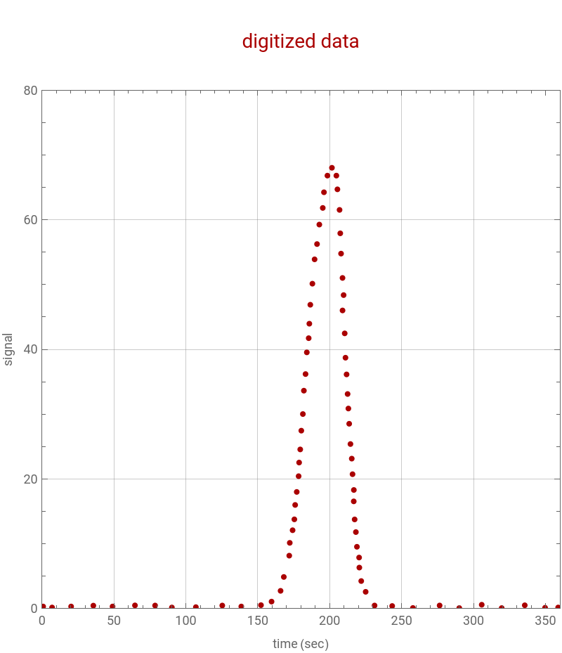
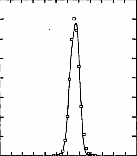
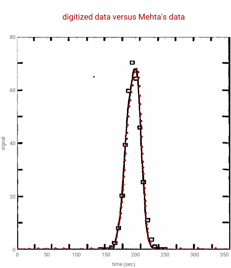
Fig. 1 from Mehta, Merson & McCoy (1974) gives the elution curve for NaCl on 450-μm non-porous glass beads, column length 85.0 cm, v0 = 0.185 cm/sec.This notebook digitizes this experimental elution curve (i.e., Fig. 1) and represents it using the moment / Hermite (Gram–Charlier) polynomial method of Mehta, Merson & McCoy, "Hermite Polynomial Representation of Chromatography Elution Curves," J. Chromatogr. 88 (1974) 1–6.The concentration profile c(t) is expanded as a series in Hermite polynomials (x), x = (t - μ1)/√(2μ2), with coefficients determined from the moments of the curve (eqns. 1–7 of the paper). Two independent routes to those moments are implemented and compared:
H
n
a
n
• Method 1: numerical (trapezoidal) integration of the raw digitized (t, signal) data over a chosen retention-time window, followed by reconstruction of the peak from its skewness (γ1) and excess kurtosis (γ2) via a Gram–Charlier / Hermite series (functions He3, He4, He6, gcPeak).
• Method 2: the digitized data are first interpolated to a continuous function f(t), and the same moments (m0, μ1, σ, γ1, γ2) are obtained by numerical integration (NIntegrate) of f(t), before applying the same Hermite/Gram–Charlier reconstruction.
The resulting predicted curves are overlaid on the digitized experimental points to check the fit, mirroring the “predicted points” overlay on the experimental curve shown in Fig. 1 of the original paper.
In[]:=
data={{{0.781664,0.302376},{7.00472,0.151188},{20.2392,0.302376},{35.6837,0.437892},{49.0364,0.302376},{64.6175,0.475113},{78.6152,0.453564},{90.283,0.151188},{106.957,0.203932},{125.313,0.453564},{138.541,0.302376},{152.224,0.512694},{159.572,1.05832},{165.835,2.72138},{168.093,4.86442},{171.87,8.15232},{172.227,10.1296},{174.197,12.0785},{175.421,13.7581},{175.982,15.9819},{177.071,17.9914},{178.383,20.4216},{178.729,22.527},{179.503,24.5531},{180.254,27.4504},{181.339,30.0147},{182.037,33.6247},{183.191,36.1868},{184.08,39.5371},{185.382,41.7279},{185.833,43.9619},{186.515,46.8893},{187.959,50.1407},{189.482,53.8995},{191.181,56.2573},{192.777,59.2657},{195.169,61.8359},{196.001,64.2549},{198.393,66.8251},{201.533,68.0346},{204.619,66.8251},{205.351,64.7084},{206.837,61.5335},{207.333,57.9158},{207.88,54.7831},{208.894,51.0288},{208.911,46.0086},{209.657,48.3801},{210.418,42.47},{210.952,38.7134},{211.72,36.1339},{212.431,33.1102},{212.972,30.8673},{213.537,28.5161},{214.415,25.3842},{215.322,23.1317},{215.862,20.728},{216.699,16.5354},{216.771,18.2937},{217.323,13.7463},{218.183,11.7927},{218.911,9.52484},{220.431,7.86177},{220.586,6.31143},{221.907,4.23326},{224.983,2.57019},{231.162,0.453564},{243.427,0.381609},{257.822,0.0769135},{276.398,0.460254},{290.052,0.0635849},{305.664,0.575021},{319.54,0.0601488},{335.585,0.491863},{349.714,0.111047},{358.797,0.151188}}};
In[]:=
data=MovingAverage[data,{10}]
Out[]=
{{{0.781664,0.302376},{7.00472,0.151188},{20.2392,0.302376},{35.6837,0.437892},{49.0364,0.302376},{64.6175,0.475113},{78.6152,0.453564},{90.283,0.151188},{106.957,0.203932},{125.313,0.453564},{138.541,0.302376},{152.224,0.512694},{159.572,1.05832},{165.835,2.72138},{168.093,4.86442},{171.87,8.15232},{172.227,10.1296},{174.197,12.0785},{175.421,13.7581},{175.982,15.9819},{177.071,17.9914},{178.383,20.4216},{178.729,22.527},{179.503,24.5531},{180.254,27.4504},{181.339,30.0147},{182.037,33.6247},{183.191,36.1868},{184.08,39.5371},{185.382,41.7279},{185.833,43.9619},{186.515,46.8893},{187.959,50.1407},{189.482,53.8995},{191.181,56.2573},{192.777,59.2657},{195.169,61.8359},{196.001,64.2549},{198.393,66.8251},{201.533,68.0346},{204.619,66.8251},{205.351,64.7084},{206.837,61.5335},{207.333,57.9158},{207.88,54.7831},{208.894,51.0288},{208.911,46.0086},{209.657,48.3801},{210.418,42.47},{210.952,38.7134},{211.72,36.1339},{212.431,33.1102},{212.972,30.8673},{213.537,28.5161},{214.415,25.3842},{215.322,23.1317},{215.862,20.728},{216.699,16.5354},{216.771,18.2937},{217.323,13.7463},{218.183,11.7927},{218.911,9.52484},{220.431,7.86177},{220.586,6.31143},{221.907,4.23326},{224.983,2.57019},{231.162,0.453564},{243.427,0.381609},{257.822,0.0769135},{276.398,0.460254},{290.052,0.0635849},{305.664,0.575021},{319.54,0.0601488},{335.585,0.491863},{349.714,0.111047},{358.797,0.151188}}}
In[]:=
p=ListPlot[data,GridLines->Automatic,Frame->True,AspectRatio->1,PlotStyle->{Darker@Red,Dashed,Thick},PlotRange->{{0,360},{0,80}},Frame->True,FrameLabel->{"time (sec)","signal"},PlotLabel->Style["\ndigitized data\n",Darker@Red,14],AspectRatio->1,ImageSize->400]
Out[]=
In[]:=
IMG=
;
In[]:=
Show[p,Prolog->{Raster[ImageData[IMG,DataReversed->True],{Scaled[{0.0,0.0}],Scaled[{1,1}]}]},PlotLabel->Style["\ndigitized data versus Mehta's data\n",Darker@Red,14]]
Out[]=
Method 1
Method 1
In[]:=
tdata=Transpose[Flatten[data,1]][[1]]
Out[]=
{0.781664,7.00472,20.2392,35.6837,49.0364,64.6175,78.6152,90.283,106.957,125.313,138.541,152.224,159.572,165.835,168.093,171.87,172.227,174.197,175.421,175.982,177.071,178.383,178.729,179.503,180.254,181.339,182.037,183.191,184.08,185.382,185.833,186.515,187.959,189.482,191.181,192.777,195.169,196.001,198.393,201.533,204.619,205.351,206.837,207.333,207.88,208.894,208.911,209.657,210.418,210.952,211.72,212.431,212.972,213.537,214.415,215.322,215.862,216.699,216.771,217.323,218.183,218.911,220.431,220.586,221.907,224.983,231.162,243.427,257.822,276.398,290.052,305.664,319.54,335.585,349.714,358.797}
In[]:=
ydata=Transpose[Flatten[data,1]][[2]]
Out[]=
{0.302376,0.151188,0.302376,0.437892,0.302376,0.475113,0.453564,0.151188,0.203932,0.453564,0.302376,0.512694,1.05832,2.72138,4.86442,8.15232,10.1296,12.0785,13.7581,15.9819,17.9914,20.4216,22.527,24.5531,27.4504,30.0147,33.6247,36.1868,39.5371,41.7279,43.9619,46.8893,50.1407,53.8995,56.2573,59.2657,61.8359,64.2549,66.8251,68.0346,66.8251,64.7084,61.5335,57.9158,54.7831,51.0288,46.0086,48.3801,42.47,38.7134,36.1339,33.1102,30.8673,28.5161,25.3842,23.1317,20.728,16.5354,18.2937,13.7463,11.7927,9.52484,7.86177,6.31143,4.23326,2.57019,0.453564,0.381609,0.0769135,0.460254,0.0635849,0.575021,0.0601488,0.491863,0.111047,0.151188}
trapz[x_,y_]:=Total[(y[[1;;-2]]+y[[2;;-1]])/2*Differences[x]];He3[z_]:=z^3-3z;He4[z_]:=z^4-6z^2+3;He6[z_]:=z^6-15z^4+45z^2-15;gcPeak[t_,area_,mean_,sd_,g1_,g2_]:=Module[{z,phi},z=(t-mean)/sd;phi=PDF[NormalDistribution[0,1],z];(area/sd)phi(1+(g1/6)He3[z]+(g2/24)He4[z]+(g1^2/720)He6[z])];
Per-peak moment analysis + Gram-Charlier reconstruction
peakResults=Module[{lo,hi,mask,tw,yw,m0,mu1,m2,m3,m4,sigma,gamma1,gamma2,gc,tp,t},{lo,hi}={150,230};mask=(#>=lo&&#<=hi)&/@tdata;tw=Pick[tdata,mask];yw=Pick[ydata,mask];m0=trapz[tw,yw];mu1=trapz[tw,twyw]/m0;m2=trapz[tw,(tw-mu1)^2yw]/m0;m3=trapz[tw,(tw-mu1)^3yw]/m0;m4=trapz[tw,(tw-mu1)^4yw]/m0;sigma=Sqrt[m2];gamma1=m3/sigma^3;gamma2=m4/sigma^4-3;tp=Table[x,{x,120,270}];gc=gcPeak[tp,m0,mu1,sigma,gamma1,gamma2];<|"Window"->{lo,hi},"tp"->tp,"y"->yw,"m0"->m0,"mu1"->mu1,"sigma"->sigma,"gamma1"->gamma1,"gamma2"->gamma2,"PlateNumber"->mu1^2/m2,"GC"->gc|>];
7. Overlay plot: raw data vs per-peak Gram-Charlier reconstructions
Method 2
Method 2
References
References
R. V. Mehta, R. L. Merson and B. J. McCoy, "Hermite Polynomial Representation of Chromatography Elution Curves," Journal of Chromatography, 88 (1974) 1–6. (Source of the digitized elution curve, Fig. 1, and of the moment / Hermite-series method implemented in this notebook.)
1. M. Kubin, Collect. Czech. Chem. Commun., 30 (1965) 1104, 2900.
2. E. Kucera, J. Chromatogr., 19 (1965) 237.
3. P. Schneider and J. M. Smith, Amer. Inst. Chem. Eng. J., 14 (1968) 762.
4. M. Suzuki and J. M. Smith, Chem. Eng. Sci., 26 (1971) 221.
5. J. C. Adrian and J. M. Smith, J. Catal., 18 (1970) 57.
6. R. V. Mehta, R. L. Merson, and B. J. McCoy, Amer. Inst. Chem. Eng. J., 19 (1973) 1068.
7. O. Levenspiel and W. K. Smith, Chem. Eng. Sci., 6 (1957) 227.
8. R. Courant and D. Hilbert, Methods of Mathematical Physics, Vol. I, Interscience, New York, 1953, pp. 91–93.
9. R. V. Mehta, M.S. Thesis, Dept. of Chem. Eng., Univ. Calif., Davis, Calif., 1973.
CITE THIS NOTEBOOK
CITE THIS NOTEBOOK
Hermite polynomial representation of chromatography elution curves
by Housam Binous
Wolfram Community, STAFF PICKS, August 17, 2026
https://community.wolfram.com/groups/-/m/t/3781869
by Housam Binous
Wolfram Community, STAFF PICKS, August 17, 2026
https://community.wolfram.com/groups/-/m/t/3781869