The whole post in one animation. Left: Monte Carlo points scattered at random clump and leave gaps. Right: Sobol’ low-discrepancy points fill the same square evenly. Below: the error of a sample integral as the points accumulate — Monte Carlo crawls down the 1/√N line while Sobol’ plunges along 1/N. Generated near the end of this post with one call to heroAnimation[].
Almost every number a Bayesian reports — a posterior mean, a credible interval, a predicted drug concentration — is secretly an integral over the space of unknown parameters. This post is about computing those integrals up to an order of magnitude more cheaply.
The default tool is Monte Carlo: average the integrand over random samples. It is universal and assumption-free, but its error shrinks only as — one more correct digit costs a hundred times more samples. Quasi-Monte Carlo (QMC) keeps the same averaging but replaces the random sample with a deterministic low-discrepancy sequence (Sobol’, Halton) engineered to fill space evenly. For smooth integrands the error then falls almost as fast as — nearly a full power of N better.
-1/2
N
O
-1
N
d
(logN)
We test that promise on a genuine inference problem: a six-parameter pharmacokinetic model fit to the classic Theophylline data. We build Halton and Sobol’ from scratch, set up the posterior, contrast it with classical curve-fitting, and measure the convergence. The headline, on a real-data posterior: Monte-Carlo slopes near against Sobol’ slopes near , and a 2×–18× saving in expensive model evaluations.
-0.5
-0.95
How to read this: every section opens with the plain idea, then the equations, the runnable Wolfram Language, and the measured numbers. All figures are pre-rendered — the post reads straight through — and every code cell runs if you load the attached package.
Setup
Setup
Skip this if you only want to read. To run the code, put the attached package qmc_bayes_helpers.wl next to the notebook and evaluate the three cells below once. They define the generators, the pharmacokinetic model, the data, the priors, and the posterior that every later section reuses.
SetDirectory[NotebookDirectory[]];Get["qmc_bayes_helpers.wl"];
(*Lognormal-priormediansandlog-scaleSDsfor{ka,CL,V1,Q,V2,sigma}*)priorMedians={1.5,3.0,35.0,2.0,25.0,1.0};priorLogSD={0.6,0.5,0.5,0.7,0.7,0.5};(*Realdata:TheophyllineSubject1(single320mgoraldose)*)theoph=LoadTheoph[];subj1=SelectSubject[theoph,1];
(*TheBayesianproblemanditsLaplace-Gaussianposterior*)pkProblem=BayesProblem[subj1["dose"],subj1["t"],subj1["c"],priorMedians,priorLogSD];pkLaplace=LaplacePosterior[pkProblem];
1. The square-root wall
1. The square-root wall
Want the average of something over a space too big to enumerate? Sample it. Throw N random points, average the values. This Monte-Carlo estimate works in any dimension with no smoothness assumptions — which is why it is everywhere. The price is the error,
ϵ
MC
σ(f)
N
-1/2
N
Halving the error means quadrupling the work; one more decimal digit costs a hundredfold. When each sample is an expensive model solve, that square-root wall is the entire problem. Its cause is visible: random points clump and leave gaps, wasting information. What if we placed them on purpose?
mc=LDPoints["MonteCarlo",256,2];hal=LDPoints["Halton",256,2];sob=LDPoints["Sobol",256,2];GraphicsRowListPlot#,&/@{mc,hal,sob}
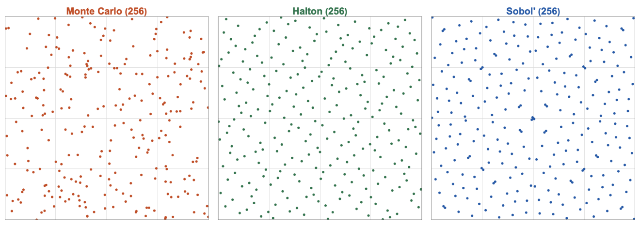
Figure 1. 256 points in the unit square. Monte Carlo (left) clumps and leaves holes; Halton (centre) and Sobol’ (right) lay down an even, gap-free pattern.
2. Low-discrepancy sequences
2. Low-discrepancy sequences
A low-discrepancy sequence fills the cube as evenly as possible at every scale. Halton uses the radical inverse of the index in a different prime base per coordinate; Sobol’ is a base-2 digital net built from "direction numbers" (we use the Joe–Kuo tables). Both are a few lines, both are in the attached package. Their L₂ star discrepancy — the root-mean-square box-vs-volume mismatch by Warnock’s exact formula, a cheap proxy for the L∞ discrepancy in the theorem below — decays like for random points but nearly for these sequences:
-1/2
N
-1
N
Nvals=2^Range[4,12];dMC=Mean[Table[StarDiscrepancyL2[RandomizedLDPoints["MonteCarlo",#,2,100r+#]],{r,20}]]&/@Nvals;dHal=StarDiscrepancyL2[LDPoints["Halton",#,2]]&/@Nvals;dSob=StarDiscrepancyL2[LDPoints["Sobol",#,2]]&/@Nvals;ListLogLogPlot[{Transpose[{Nvals,dMC}],Transpose[{Nvals,dHal}],Transpose[{Nvals,dSob}]},Joined->True,Mesh->All]
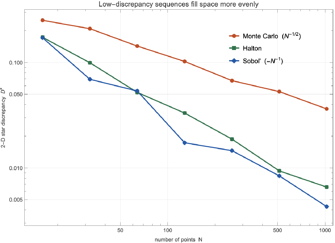
Figure 2. L₂ star discrepancy versus N (log-log). Monte Carlo rides the line; Halton and Sobol’ track .
-1/2
N
-1
N
The theorem behind it. For an integrand f of bounded variation (Hardy–Krause), the Koksma–Hlawka inequality splits the QMC error into the function’s variation times the points’ discrepancy:
V(f)
1
N
N
∑
n=1
x
n
*
D
N
With =O — this being the L∞ (supremum) star discrepancy, of which Figure 2 plots the cheaper L₂ proxy — QMC inherits that rate, provided the integrand is smooth enough to have finite variation. That proviso drives every modelling choice below.
*
D
N
-1
N
d
(logN)
*
D
N
3. The model: a drug moving through the body
3. The model: a drug moving through the body
What happens when you take a pill. The drug dissolves in the gut and is absorbed into the bloodstream; the blood carries it to the tissues, where some of it parks reversibly; meanwhile the liver and kidneys clear it away. Plot the blood concentration against time and you get a familiar shape: a fast rise to a peak, then a slow decline. Pharmacokinetics is the quantitative description of that curve, and it is the backbone of every dosing decision — how much, how often, and how confident we are.
We use the canonical teaching data set, Theophylline (an anti-asthma drug, from Boeckmann, Sheiner & Beal): 12 subjects, each a single oral dose, serum concentration sampled 11 times over ~25 h. Theophylline has a narrow therapeutic window (about 10–20 mg/L; toxicity climbs above it), so getting the curve — and its uncertainty — right genuinely matters.
3.1 The two-compartment system
3.1 The two-compartment system
The standard structural model splits the body into two well-mixed compartments: a central one (blood and richly-perfused organs, volume ) where we actually measure concentration, and a peripheral one (slower tissues, volume ). The swallowed dose sits in a gut depot and is absorbed first-order into the central compartment; drug shuttles between central and peripheral, and is cleared from the central compartment. Writing the amounts in each compartment, the dynamics are a linear system of ODEs:
V
1
V
2
A
g
A
g
t
k
a
A
g
A
1
t
k
a
A
g
CL
V
1
A
1
Q
V
1
A
1
Q
V
2
A
2
A
2
t
Q
V
1
A
1
Q
V
2
A
2
with the oral dose as initial condition (0)=D, (0)=(0)=0, and the measured concentration .
A
g
A
1
A
2
C(t)=/
A
1
V
1
3.2 The six parameters, one by one
3.2 The six parameters, one by one
These are the unknowns we infer — each a physical quantity a clinician can interpret:
◼
ka — absorption rate (1/h). How fast the drug leaves the gut for the blood; it sets the steepness of the rising limb and the time-to-peak.
◼
CL — clearance (L/h). Volume of blood completely cleared of drug per hour. It alone fixes the total exposure — the single most important dosing parameter.
AUC=D/CL
◼
V1 — central volume (L). Relates dose to the initial concentration; small means a high peak.
V
1
◼
Q — inter-compartmental clearance (L/h). How fast drug exchanges with the tissues; it shapes the bend between the fast and slow phases.
◼
V2 — peripheral volume (L). How much drug the tissues hold; it stretches the slow elimination tail.
◼
σ — residual scatter (mg/L). The combined assay-plus-model noise on each measurement — itself an unknown to be estimated.
From these follow the quantities dosing actually turns on: half-life ∝/CL, exposure , peak concentration, and the steady state reached under repeated dosing.
t
1/2
V
1
D/CL
3.3 A closed form — no solver needed
3.3 A closed form — no solver needed
Because the system is linear, it has an exact solution: a sum of three exponentials in the macro-rate constants α, β (the eigenvalues of the compartment matrix) and . This makes each likelihood evaluation a handful of Exps rather than an ODE solve:
k
a
C(t)=D++
k
a
V
1
A
α
-αt
e
A
β
-βt
e
A
k
-t
k
a
e
(*Theclosed-formconcentration;ka,CL,V1,Q,V2,dose.*)Plot[PKConcentration[t,{1.5,2.8,30.,2.0,20.},320.],{t,0,25},Frame->True,FrameLabel->{"time (h)","conc (mg/L)"},PlotStyle->RGBColor[0.153,0.51,0.64]]
Why bother with six parameters? A simpler one-compartment model has three. The second compartment is what lets the curve bend — a fast distribution phase then a slow elimination phase — which real drugs do. The cost is that the two tissue parameters (Q, V2) are only weakly pinned down by a single subject’s sparse samples. Holding honest uncertainty about them, rather than a false-precision point estimate, is exactly where the Bayesian treatment earns its keep.
4. The Bayesian model, and why it is all integrals
4. The Bayesian model, and why it is all integrals
Each measurement is the model prediction plus Gaussian scatter, =C()+ with ∼N(0,). All six parameters are positive, so each gets a lognormal prior (a normal prior on its logarithm). Bayes’ rule gives the posterior:
c
i
t
i
ϵ
i
ϵ
i
2
σ
Now the key point. Everything we want from this posterior is an expectation — an integral over the six-dimensional parameter space:
5. Classical curve-fitting versus the Bayesian posterior
5. Classical curve-fitting versus the Bayesian posterior
The classical reflex. Hand this data to a statistician and the first move is nonlinear least squares — in Wolfram Language, NonlinearModelFit — which slides the six parameters until the squared residuals are smallest. It is fast and gives a tidy best-fit curve:
Figure 3. Same data, two philosophies. Left: least squares returns a single best-fit curve — and, because the model is unidentifiable here, no usable error band. Right: the Bayesian posterior (sampled by QMC) delivers a full predictive band; the lognormal priors gently regularize the directions the data cannot constrain.
The Bayesian posterior fixes this honestly: the priors keep the weakly-identified directions finite, and the answer is a full joint distribution — every parameter, every prediction, with calibrated uncertainty. The catch is the one from §4: you must integrate. The options:
◼
Laplace approximation — fit a Gaussian at the posterior mode; cheap, and the basis we build on here.
QMC does not compete with MCMC so much as complement it: where you can reparameterize the posterior to be smooth and roughly Gaussian (Bayesian asymptotics says you usually can), QMC integration buys back most of the lost power. That is the recipe we follow next.
6. The fit
6. The fit
Figure 4. Theophylline Subject 1: the 11 measurements with the 90% posterior-predictive band. The fit captures the absorption peak near 2 h and the slow elimination tail.
Is the Gaussian approximation good enough? We check against the full posterior via importance sampling (FitProposal + ImportanceEstimate): in our runs the well-identified parameters agree to ~10%. And the convergence demonstration does not depend on the approximation being perfect — only on the integrand we actually integrate being smooth, which it is.
7. The convergence law
7. The convergence law
That is the headline, on a real-data posterior: at a fixed budget of model solves Sobol’ reaches roughly 50× lower error than Monte Carlo at N = 32768 — about 1.7 extra correct digits — and the gap keeps widening. The result rides on the integrand being smooth (§6), not on the Gaussian being exact.
8. Why dimension matters
8. Why dimension matters
9. Does it recover the truth?
9. Does it recover the truth?
A fast wrong answer is worthless, so we generate data from known parameters, fit, and check the posterior brackets them (on a deliberately denser time grid than the real 11-point design, to isolate parameter recovery from data sparsity):
10. The practical pay-off
10. The practical pay-off
That is the value proposition in one figure. QMC changes neither the model nor the estimand — only which points you evaluate at — and that single swap buys back most of an order of magnitude in expensive model runs.
11. The cover animation
11. The cover animation
12. Conclusions
12. Conclusions
When QMC helps, and when it does not. It helps when the dimension is low-to-moderate or the effective dimension is small, the integrand is smooth, and evaluations are the bottleneck. It does not help for rough or discontinuous integrands, very high dimension, or heavy-tailed importance weights — which is why we integrate against a smooth Gaussianized posterior rather than a spiky ratio.
The portable recipe. (1) reparameterize to an unconstrained space and build a Gaussian approximation of the posterior; (2) map the unit cube through it with the inverse-CDF transform; (3) swap your pseudo-random draws for a randomized Sobol’ or Halton set; (4) average over a few randomizations for an error bar. Two lines of change, most of an order of magnitude back.
13. References & reproducibility
13. References & reproducibility
Halton, J. H. (1960). Numerische Mathematik 2, 84–90. • Sobol’, I. M. (1967). USSR Comp. Math. Math. Phys. 7, 86–112. • Joe, S., & Kuo, F. Y. (2008). SIAM J. Sci. Comput. 30, 2635–2654 (the direction numbers used here).
Niederreiter, H. (1992). Random Number Generation and Quasi-Monte Carlo Methods, SIAM. • Caflisch, R. E. (1998). Acta Numerica 7, 1–49 (effective dimension). • Owen, A. B. (1998). J. Complexity 14, 466–489 (randomized QMC). • Gerber, M., & Chopin, N. (2015). JRSS B 77, 509–579 (QMC in Bayesian computation).
Boeckmann, Sheiner & Beal (1994). NONMEM Users Guide (the Theophylline data). • Gabrielsson & Weiner (2016). Pharmacokinetic and Pharmacodynamic Data Analysis (the two-compartment model).
All code is pure Wolfram Language at github.com/mthiel74/QuasiMonteCarloBayesianEstimation (https://github.com/mthiel74/QuasiMonteCarloBayesianEstimation). The companion package qmc_bayes_helpers.wl is the single source of truth; the figure scripts and this notebook both load it. To rebuild:
wolframscript -file wolfram/fetch_theoph.wls # real data -> data/
wolframscript -file wolfram/run_all.wls # all figures -> docs/images/
wolframscript -file community/build_notebook.wls
wolframscript -file wolfram/run_all.wls # all figures -> docs/images/
wolframscript -file community/build_notebook.wls
Generated June 23, 2026.
CITE THIS NOTEBOOK
CITE THIS NOTEBOOK
Quasi-Monte Carlo Bayesian estimation: Sobol', Halton vs Monte Carlo, PK posterior convergence
by Marco Thiel
Wolfram Community, STAFF PICKS, July 1, 2026
https://community.wolfram.com/groups/-/m/t/3742350
by Marco Thiel
Wolfram Community, STAFF PICKS, July 1, 2026
https://community.wolfram.com/groups/-/m/t/3742350