ABSTRACT (original article): We describe a simple method for tracking solutions of nonlinear equations f(u,α) = 0 through turning points (also known as limit or saddle-node bifurcation points). Our implementation makes use of symbolic software such as Mathematica to derive an exact system of nonlinear ODE equations to follow the solution path, using a parameterization closely related to arc length. We illustrate our method with examples taken from the engineering literature, including examples that involve nonlinear boundary value problems that have been discretized by finite difference methods. Since the code requirement to implement the method is modest, we believe the method is ideal for demonstrating continuation methods in the classroom. CITATION (original article): Higgins, B. G., & Binous, H. (2010). A Simple Method for Tracking Turning Points in Parameter Space. JOURNAL OF CHEMICAL ENGINEERING OF JAPAN, 43(12), 1035–1042. DOI: https://doi.org/10.1252/jcej.10we122
Here, we provide the numerical solution(s) using Wagon’s graphical method (Ref. 2) as well as the Homotopy method described thoroughly in Ref. 1.
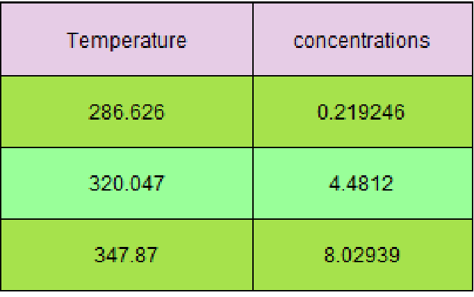
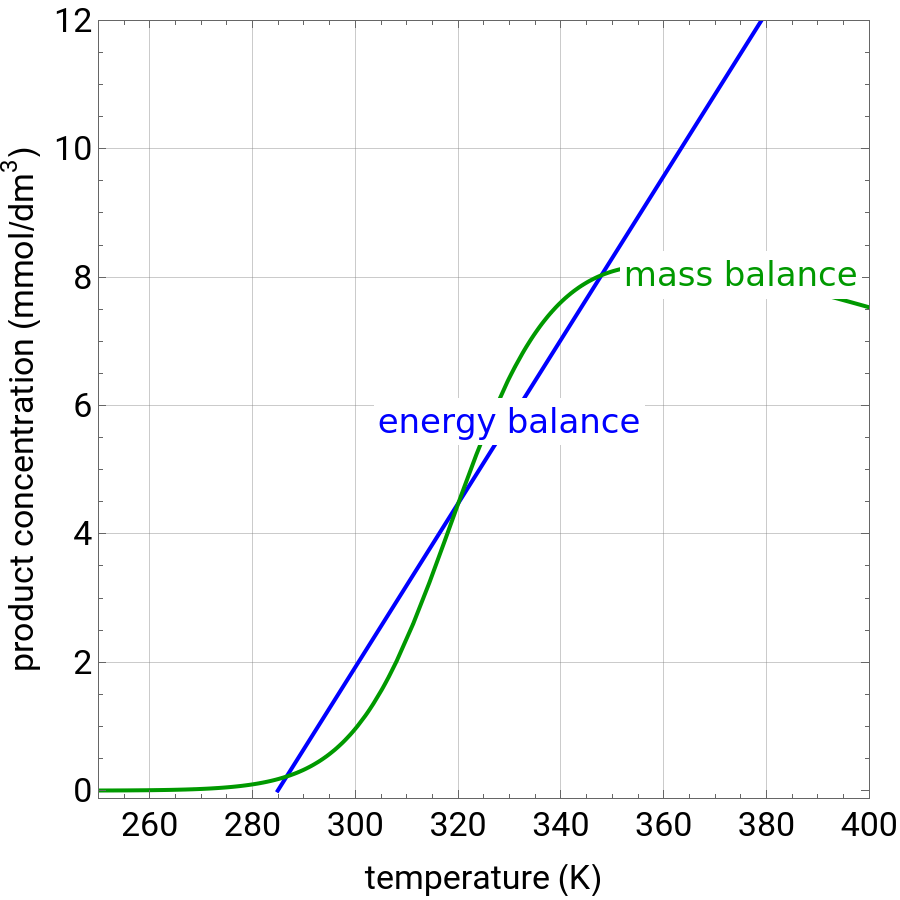
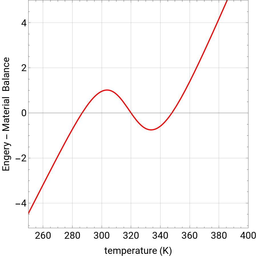
Let us consider a continuous stirred-tank reactor (CSTR) with heat transfer. The reversible, elementary, exothermic reaction takes place in the CSTR. The feed temperature, residence time, heat transfer coefficient, and reverse-reaction pre-exponential factor are set as follows:We determine the steady-state concentration of product and reactor the temperature by solving the mass and energy balances. The intersections of the green curve and straight blue line correspond to the steady-state solutions for the CSTR. Either one or three solutions are possible; for three solutions, the middle solution is unstable.
A↔B
V=50000,kf=1.×,Ef=20000,Er=24000,R=1.987,ρ=0.8,Cp=2,cA0=0.01,A=8.94,ΔHrxn=-15000,Tc=310,v=100,U=3.5,kr=5.×andτ=400
11
10
12
10
B
The mass balance is nonlinear:=τ1+τ+τ,where is the concentration of product (), is the reactant feed concentration (mol), and are the pre-exponential factors for the forward and reverse reactions (1/s), and are the activation energies for the forward and reverse reactions (cal/mol), is residence time (s), is the ideal gas constant (cal/[mol K]), and is temperature of the CSTR (K).The energy balance is linear and has two terms that correspond to (1) the energy needed to change the feed temperature to the reactor temperature, and (2) the energy removed or added by heat transfer to a cooling/heating fluid, which is at a constant temperature of 310 K. = ,where is the volumetric flow rate (/s), is the density of the bulk fluid (), is the mass heat capacity of the feed (cal/[kg K]), and are the temperatures of the feed and coolant (K), is the heat transfer coefficient (), is the heat transfer area (), and is the heat of reaction (cal/mol).
C
B
k
f
-
E
f
RT
e
C
A,0
k
f
-
E
f
RT
e
k
r
-
E
r
RT
e
C
B
B
mol/
3
dm
C
A,0
k
f
k
r
E
f
E
r
τ
R
T
C
B
-vρCp(T-)-UA(T-)
T
0
T
c
vΔH
v
3
dm
ρ
kg
3
dm
Cp
T
0
T
c
U
cal/[Ks]
2
dm
A
2
dm
ΔH
Case 1: Three steady-states obtained for Tf=280K
Case 1: Three steady-states obtained for
Tf=280K
As the feed temperature increases from a low value, the reactor temperature increases until the reactor reaches a temperature above which three steady-state solutions are possible. The upper and lower solutions are stable, and the middle solution is unstable. The operating conditions of the reactor depend on how the reactor is started up.
Case 2: Single steady-state obtained for Tf=295K
Case 2: Single steady-state obtained for
Tf=295K
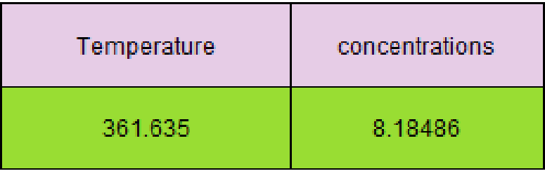
As the feed temperature increases further, a temperature is reached above which only one solution is possible, and this has a high conversion.Varying the heat transfer coefficient changes both the slope and intercept of the energy balance line, and this can change the number of steady-state solutions. Increasing the pre-exponential factor for the reverse reaction changes the mass balance curve, and the maximum conversion decreases as the equilibrium conversion become less than one.
Graphical Method by Wagon
Graphical Method by Wagon
Case 1
Case 1
In[]:=
V=50000;kf=1*^11;Ef=20000;Er=24000;R=1.987;ρ=0.8;Cp=2;cA0=0.01;A=8.94;ΔHrxn=-15000;Tc=310;v=100;U=3.5;kr=5*^12;Tf=280;τ=400;ebal[T_]:=-*1000;mbal[T_]:=*1000;plt1=Plot[{ebal[T],mbal[T]},{T,250,400},PlotStyle{{Thick,Blue},{Thick,RGBColor[0,0.6,0]}},PlotRange{{250,400},{0,0.012*1000}},PlotRangePadding{None,{Scaled@0.01,None}},FrameTrue,FrameTicksTrue,FrameLabel{"temperature (K)",Row@{"product concentration (mmol/",Superscript["dm",3],")"}},LabelStyle{17,Black},ImageSize{450,450},AspectRatioFull,Epilog{Text[Framed[Style[Row@{#1," balance"},17,#2],BackgroundWhite,FrameStyleNone,FrameMarginsTiny],#3]&@@@{{"energy",Blue,{If[Tf≤270,290,330],ebal@If[Tf≤270,290,330]}},{"mass",RGBColor[0,0.6,0],{375,mbal@375}}}},GridLinesAutomatic]
v*ρ*Cp*(T-Tf)+U*A*(T-Tc)
v*ΔHrxn
τ*kf*Exp-*cA0
Ef
R*T
1+τ*kf*Exp-+τ*kr*Exp-
Ef
R*T
Er
R*T
Out[]=
In[]:=
plt=Plot[ebal[T]-mbal[T],{T,250,400},PlotStyle{Thick,Red},PlotRange{{250,400},{-5,5}},PlotRangePadding{None,{Scaled@0.01,None}},FrameTrue,FrameTicksTrue,FrameLabel{"temperature (K)","Engery - Material Balance"},LabelStyle{17,Black},ImageSize{450,450},AspectRatioFull,GridLinesAutomatic]
Out[]=
In[]:=
tbl=First[Cases[plt,x_LineFirst@x,Infinity]];
In[]:=
tbl2=Table[tbl[[i,1]],{i,1,Length[tbl]}];
In[]:=
signs=Sign[Map[ebal,tbl2]-Map[mbal,tbl2]];
Case 2
Case 2
Homotopy Method by Higgins and Binous (Ref. 1)
Homotopy Method by Higgins and Binous (Ref. 1)
Case 1
Case 1
s is a continuation parameter
WhenEvent keeps track of the molar volumes obtained for t=1
Case 2
Case 2
s is a continuation parameter
WhenEvent keeps track of the molar volumes obtained for t=1
Acknowledgement
Acknowledgement
This problem and its description are largely inspired by the following WWW page: https://demonstrations.wolfram.com/MultipleSteadyStatesInAContinuouslyStirredTankReactor/
References
References
◼
[1] Higgins, B. G., & Binous, H. (2010). A Simple Method for Tracking Turning Points in Parameter Space. JOURNAL OF CHEMICAL ENGINEERING OF JAPAN, 43(12), 1035–1042. DOI: https://doi.org/10.1252/jcej.10we122
◼
[2] S. Wagon, Mathematica in Action: Problem Solving through Visualization and Computation, 3rd ed., Berlin: Springer–Verlag, 2010.
CITE THIS NOTEBOOK
CITE THIS NOTEBOOK
Multiple steady states in a continuously stirred tank reactor: graphical and homotopy solutions
by Housam Binous and Ahmed Bellagi
Wolfram Community, STAFF PICKS, July 3, 2025
https://community.wolfram.com/groups/-/m/t/3490572
by Housam Binous and Ahmed Bellagi
Wolfram Community, STAFF PICKS, July 3, 2025
https://community.wolfram.com/groups/-/m/t/3490572