Introduction
Introduction
Traditionally control design is based on a mathematical model of the system.
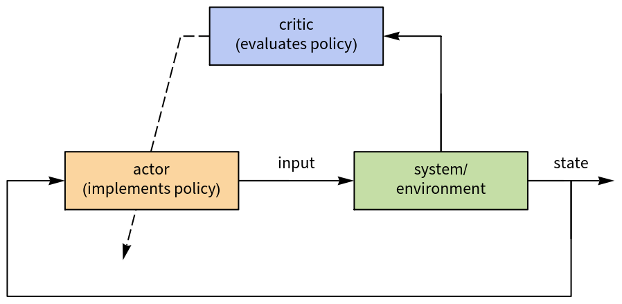
Using Reinforcement Learning, controllers can be designed without a mathematical model. This is done by interacting with a simulation model or maybe even the physical system.
In this approach, inputs are applied to the system, evaluated, and the control or policy updated to minimize a quality function Q.
Model
Model
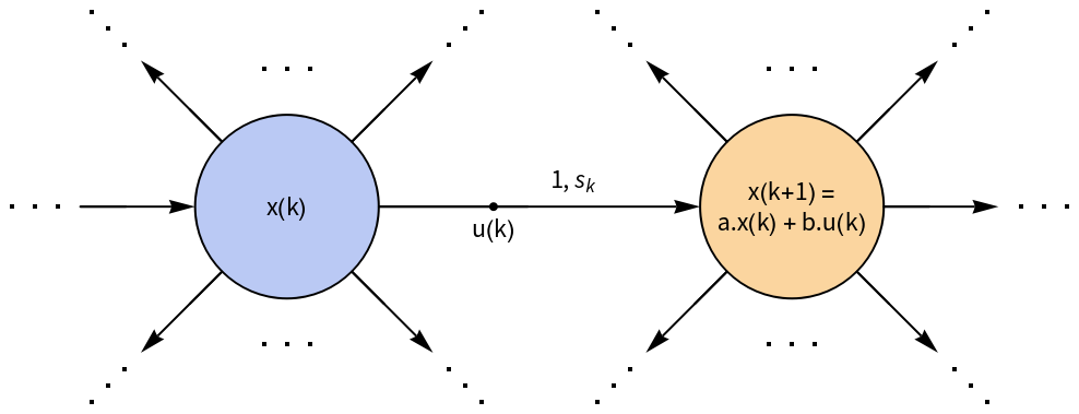
The model of the system (or environment) is unknown but is assumed to be discrete-time linear time-invariant (LTI). (1)Here is the state vector and is the input vector.
x(k+1)=a.x(k)+b.u(k)
x∈
n
u∈
m
Define the stage cost to be quadratic =x(k).q.x(k)+u(k).r.u(k).
s
k
Define the performance index as the infinite-horizon sum = =x(k).q.x(k)+u(k).r.u(k) (2)
J
k
∞
∑
i=k
s
k
J
k
∞
∑
i=k
A discrete-time LTI is a Markov Decision Processes (MDP) where the set of states is , the set of actions is , the transition probabilities are 1, and the cost function is .
X=
n
U=
m
s
k
Value of a policy
Value of a policy
Let’s assume a stationary optimal policy . This is the constant state feedback optimal control law.
u(k)=-g.x(k)
Then from (1) (3)
x(k+1)=(a-b.g).x(k),x(k+2)=(a-b.g).x(k+1)=.x(k),⋮
2
(a-b.g)
x(k+n)=.x(k)
n
(a-b.g)
The value of a policy is the cost accrued by following a policy. Denote by (x(k)) the value of the policy . It is also denoted by .
J
k
V
g
u(k)=-g.x(k)
g
J
k
From (2)(x(k))=x(i).q.x(i)+x(i)g.r.g.x(i) (4)(x(k))=x(i).(q+g.r.g).x(i) (x(k))=x(k).(q+g.r.g).x(k)+x(k+1).(q+g.r.g).x(k+1)+… Using (3)(x(k))=x(k).(q+g.r.g).x(k)+x(k)(a-b.g).(q+g.r.g).(a-b.g).x(k)+… (x(k))=x(k).I+(a-b.g)++….(q+g.r.g).I+(a-b.g)++….x(k)(x(k))=x(k)..x(k) (5)
V
g
∞
∑
i=k
V
g
∞
∑
i=k
V
g
V
g
V
g
2
(a-b.g)
2
(a-b.g)
V
g
P
g
The value is quadratic and positive definite. From any initial value the policy drives the system to the origin along the surface.
V
g
u(k)=-g.x(k)
V
g

It can be shown that the solution of the discrete-time algebraic Riccati equation (DARE) for the linear quadratic regulation (LQR) problem to minimize x(k).q.x(k)+u(k).r.u(k) for corresponds to the optimal policy
P
g
∞
∑
i=0
x(k+1)=a.x(k)+b.u(k)
u(k)=-g.x(k)
The Q function of a policy
The Q function of a policy
Define the quality function Q to be the cost to start in state and use an arbitrary input signal at instant k, and for all subsequent instants.
x(k)
u(k)
u(i)=-g.x(i),i>k
Q(x(k),u(k))=x(k).q.x(k)+u(k).r.u(k)+x(i).q.x(i)+x(i)g.r.g.x(i)
∞
∑
i=k+1
V
ℊ
Q(x(k),u(k))=x(k).q.x(k)+u(k).r.u(k)+(x(k+1))
V
g
Q(x(k),u(k))=x(k).q.x(k)+u(k).r.u(k)+x(k+1)..x(k+1)
P
g
Q(x(k),u(k))=x(k).q.x(k)+u(k).r.u(k)+(x(k)a+u(k).b)..(a.x(k)+b.u(k))
P
g
Q(x(k),u(k))=
.
.
x(k) |
u(k) |
q+a. P g | a. P g |
b. P g | r+b. P g |
x(k) |
u(k) |
It can be shown that computing the input that minimizes using ==0 gives the solution of the LQR problem
u(k)
Q(x(k),u(k))
∂Q(x(k),u(k))
∂u(k)
u(k)=.b..a.x(k)
-1
(r+b..b)
P
g
P
g
However it cannot be implemented the above way because the system’s dynamics is unknown.
Let’s assume that and set ==0. This gives .x(k)+.u(k)==0and
Q(x(k),u(k))=
.
.
x(k) |
u(k) |
s xx | s xu |
s ux | s uu |
x(k) |
u(k) |
∂Q(x(k),u(k))
∂u(k)
s
ux
s
uu
u(k)==-..x(k)
-1
s
uu
s
ux
Thus we can compute the gain of the policy at instant as ., provided we know the matrix .
k
-1
s
uu
s
ux
s
Q learning
Q learning
Or how to compute the Q function and hence the optimal policy.
From (7) From (6)
Q(x(k),u(k))=x(k).q.x(k)+u(k).r.u(k)+(x(k+1))
V
g
Q(x(k),u(k))-(x(k+1))=x(k).q.x(k)+u(k).r.u(k)
V
g
Q(x(k),u(k))-Q(x(k+1),-g.x(k+1))=x(k).q.x(k)+u(k).r.u(k)
Since s is a symmetric matrix it has unique entries ,…, and can be expanded out linearly as
d=1+2+…+(n+m)
s
1
s
d
Q(x(k),u(k))
Q(x(k),u(k))=
.
.
x(k) |
u(k) |
s xx | s xu |
s ux | s uu |
x(k) |
u(k) |
Q(x(k),u(k))=ϕ(x(k),u(k)).(
)
s 1 | … | s d |
Thus
(ϕ(x(k),u(k))-ϕ(x(k+1),-g.x(k+1))).(
)=x(k).q.x(k)+u(k).r.u(k)
s 1 | … | s d |
An example
An example
Consider the following system.
Let’s assume that the system starts at 2.
Let’s define the the state and input weights to be unity, set the initial gain to 0, and compute the controller using 25 simulations.
We can get a slew of property values from the data object .
This is the computed gain.
Plotting the gain values, we see how it converged to the final value from the initial gain 0.
The plot above shows that gain was updated after every 5 simulations. This can be also be obtained as a property.
We can also see the inputs that were used to excite the system. For every 5 simulations the input gain remained the same, but the input values were different.
We can also plot the state values which shows the system being regulated to 0 from the initial value 2.
Summary
Summary
Starting from the very basics I have shown the derivation of the equations to compute an optimal controller for a system without full knowledge of its underlying dynamics. The controller is computed using a trial-and error approach and it converges to the optimal solution while simultaneously regulating the system to the origin. The approach seems to work well when the underlying model is that of a linear discrete-time system, provided the process is started with a stabilizing controller. This can be extended to handle continuous and nonlinear systems and also to solve tracking problems.
References
References
◼
F. L. Lewis, D. Vrabie and K. G. Vamvoudakis, “Reinforcement Learning and Feedback Control: Using Natural Decision Methods to Design Optimal Adaptive Controllers,” in IEEE Control Systems Magazine, vol. 32, no. 6, pp. 76-105, Dec. 2012, doi: 10.1109/MCS.2012.2214134.
CITE THIS NOTEBOOK
CITE THIS NOTEBOOK
Reinforcement learning applied feedback control
by Suba Thomas
Wolfram Community, STAFF PICKS, January 15, 2025
https://community.wolfram.com/groups/-/m/t/3356797
by Suba Thomas
Wolfram Community, STAFF PICKS, January 15, 2025
https://community.wolfram.com/groups/-/m/t/3356797