ABSTRACT (original article): The higher-order WKB Mathematica® code for computing quasinormal modes, whose accuracy was significantly enhanced through extensions to higher orders and, in particular, through the use of Pad´e resummation, has been widely employed in numerous studies over the past several years. In this work, we present an updated and optimized version of the code. The main improvement consists in expanding the effective potential in a Taylor series around its maximum, rather than evaluating the full analytic expression of the WKB formula for each specific potential. This modification leads to a substantial reduction in computation time. In cases where the effective potential is complicated and involves non-rational functions, the speed gain can reach several orders of magnitude, while preserving the accuracy of the method. CITATION (original article): Konoplya, R. A.; Matyjasek, J.; Zhidenko, A. An Efficient Higher-Order WKB Code for Quasinormal Modes and Greybody Factors. International Journal of Gravitation and Theoretical Physics 2026, 2 (1), 5. https://doi.org/10.53941/ijgtp.2026.100005.
QuietCheckImport["WKB.m",PathPrepend[$Path,NotebookDirectory[]]],;
The tortoise coordinate is defined by the function f[r].
The effective potential for the Schwarzschild-de Sitter black hole is V[r]:
s==-2 corresponds to the even (scalar) channel of gravitaional perturbations.
s==2 corresponds to the odd (scalar) channel of gravitaional perturbations. This potential has the same quasinormal spectrum as for the even channel.
s==1 is for the electromagnetic perturbations.
s==0 gives the effective potential of the test massless scalar field.
s==±1/2 gives two (isospectral) potentials for the massless Dirac field.
In[]:=
f[r_]=1--;V[r_]=f[r]Piecewise,s-2,-,s2,--1,s-,+-1,s,+(1-);
2M
r
Λ
2
r
3
72+6M+ℓ(1+ℓ)-12r(6-3ℓ-3+2Λ)
3
M
2
r
2
(-2+ℓ+)
2
ℓ
3
r
2
(-2+ℓ+)
2
ℓ
2
M
2
ℓ
2
r
3
r
2
(6M+r(-2+ℓ+))
2
ℓ
ℓ(ℓ+1)
2
r
6M
3
r
2
(ℓ+1/2)
2
r
ℓ+1/2
2
r
f[r]
3M
r
1
2
2
(ℓ+1/2)
2
r
ℓ+1/2
2
r
f[r]
3M
r
1
2
ℓ(ℓ+1)
2
r
2
s
f'[r]
r
The following function adds its number in front of each line:
In[]:=
EnumerateLines[L:{__List}]:=MapThread[Prepend,{L,L//Length//Range}];
The explicit WKB formula
The explicit WKB formula
?BasicWKBFormula
BasicWKBFormula[n,{V0,V2...}] returns square of the overtone number n; V2, V3, V4... are the values of the derivatives at the potential peak.
If you already know the derivatives of the potential you can find the righthand side of the WKB formula as
2
w
2
w
2
1
2
-V2
The higher order WKB formula needs higher derivatives to be calculated.
The third order WKB formula proposed in https://inspirehep.net/record/21079 reads:
The third order WKB formula proposed in https://inspirehep.net/record/21079 reads:
2
w
2
w
2
1
2
-V2
+-7-60+9V2V4+36V2V4
2
V3
2
+n
1
2
2
V3
2
+n
1
2
288
2
V2
1
6912
2
5
V2
1
2
-V2
-3854
V3
2
1
2
4
V3
2
V3
2
1
2
2
V3
2
V2
2
V4
2
1
2
2
V2
2
V4
2
V2
2
1
2
2
V2
3
V2
2
1
2
3
V2
Calculation of the quasinormal modes using 6th-order WKB formula
Calculation of the quasinormal modes using 6th-order WKB formula
Here r is the coordinate, 3M is the initial guess for the maximum of the potential, 0 is the mode number.
WKBQNM=Block[{order=6,M=1/2,Λ=0,s=2,ℓ=2,overtone=0},WKBFormula[order,V[r],f[r],{r,3M},overtone]]
{0.747239-0.177782,0.747009-0.177837,0.747107-0.178248,0.746324-0.178435,0.7487-0.188126,0.797699-0.176571,r1.64039}
The result of the function is the list of the QNM found with 6 - th, 5 - th, 4 - th, 3 - rd, 2 - nd order WKB formula, and the eikonal approximation. The last value is the point of the maximum of the potential.
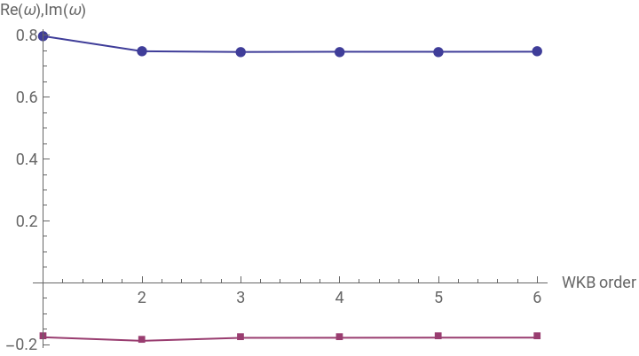
Here you can see the convergence of the WKB formula:
ListPlot[{WKBQNM//Most//Re//Reverse,WKBQNM//Most//Im//Reverse},JoinedTrue,PlotMarkersAutomatic,AxesLabel{"WKB order","Re(ω),Im(ω)"},AxesOrigin{1,0}]
In order to adjust the numerical precision, we use an extra parameter to the WKB formula:
WKBQNM=Block[{order=6,M=1/2,Λ=0,s=0,ℓ=0,overtone=0,precision=50},WKBFormula[order,V[r],f[r],{r,3M},overtone,precision]]
{0.220934036308476298738865741585280826465999-0.201632502810674961013147776104686422389378,0.21065547046438049874901724517542138454825214-0.21147080870361302071399575468949393182580757,0.219198791428453693390827557860742597236965224-0.219982467167011635500958940734548298782466689,0.2092936249463129582684041919916716911468136594-0.2303935007615620954233551421340977562097170929,0.264732162860893645361555189647692622535024260055-0.281709889430610363722382740625572732373428342710,0.3795694821839474669515511228158442221287317533232-0.1964796218578151008088891849745170855417367683804,r1.3333333333333333333333333333333333333333333333333}
For some potentials the point of the maximum is known. In these cases it is possible to put the value by hand
WKBQNM=Block[{order=6,M=1/2,Λ=0,s=1,ℓ=1,overtone=0,precision=20},WKBFormula[order,V[r],f[r],{r,3M,ThisPoint},overtone,precision]]
{0.4963828364448-0.1852740549722,0.496730173350013-0.185144502711585,0.4964674426650851-0.1844384542181891,0.49173963358176980-0.18621172962577409,0.500874836958788479-0.209147180984067067,0.5741008907838011125-0.1824706455911679973,r1.5000000000000000000}
You can also use rule in order to sunstitute the exact expression into the analytic formula
WKBQNM=Block[{order=6,Λ=0,s=1,ℓ=1,overtone=0},WKBFormula[order,V[r],f[r],r3M,overtone]]//Simplify[#,Assumptions{M>0}]&
-22932235044,,-1101114,,,(2-,r3M
112175852249
3
2
839808M
1040589792-637006529
2
139968M
3613159
2
2
5832M
5436-
6797
2
324M
151-108
2
54M
1
3
2
)3M
?WKBFormula
WKBFormula[O,V[r],f[r],rrm,n] calculates overtone n using WKB formulas up to the order O; rm is the potential peak position.WKBFormula[O,V[r],f[r],{r,r0},n,precision] calculates overtone n using WKB formulas up to the order O; r0 is the initial guess for the potential peak.
The parameter ThisPoint is just a function, that replaces FindRoot, which is used by default. You can use your own function instead:
MyRootFinder[Eq_,{R_Symbol,R0_?NumericQ},WorkingPrecisionMyPrecision_]:=NSolve[Eq,R,MyPrecision]//Cases[#,{Rx_/;Im[x]==0&&Re[x]>R0}Re[x]]&//Min//{R#}&
(here R0 is the horizon radius)
In a similar manner we can calculate also the first overtone for s=0, ℓ=2:
WKBQNM=Block[{order=6,M=1/2,Λ=0,s=0,ℓ=2,overtone={0,1},precision=20},WKBFormula[order,V[r],f[r],{r,2M,MyRootFinder},overtone,precision]]
{{0.96728376490064-0.19353217823226,0.9276934889275-0.5912538297653},{0.967312901668129-0.193526348782377,0.92771766595516-0.59123842124108},{0.9672946415463696-0.1934350575871435,0.927505084401801-0.590904801653829},{0.96642206087377966-0.19360970973912283,0.9263834433529748-0.5916202538634292},{0.967954632422429482-0.201120089473390201,0.94392200299531045-0.61872206070382931},{1.012633114482013111-0.192246450856550037,1.122192878115816288-0.520432252089796361},r1.4758574106942557113}
Here we have two dominant modes calculated with the sixth-order WKB formula:
WKBQNM//First
{0.96728376490064-0.19353217823226,0.9276934889275-0.5912538297653}
Finally, we calculate a table for all gravitational perturbations (s = 2) modes n <= ℓ <= 5 (in units M=1)
Blockorder=6,M=1,Λ=,s=2,lmax=5,precision=MachinePrecision,Table[WKBFormula[6,V[r],f[r],{r,3M},Range[0,ℓ],precision]//First,{ℓ,Abs[s],lmax}]//TableForm
1
100
0.356446-0.0854247 | 0.332943-0.261414 | 0.290057-0.453446 | |||
0.571991-0.08872 | 0.557454-0.268637 | 0.530017-0.455961 | 0.493135-0.655015 | ||
0.772061-0.089992 | 0.761189-0.271419 | 0.74019-0.457166 | 0.71066-0.649932 | 0.67495-0.851905 | |
0.965804-0.0906084 | 0.95707-0.272773 | 0.939998-0.457776 | 0.915438-0.64745 | 0.884699-0.843419 | 0.849436-1.04697 |
Higher-order WKB formula
Higher-order WKB formula
Padé approximants and averaging
Padé approximants and averaging
Grey-body factors
Grey-body factors
?WKBCoeff
WKBCoeff[O,ω^2,V[r],f[r],rrm,precision] solves the WKB formulas up to the order O for given squared frequencies ω^2 with respect to the S-matrix coefficient; rm is the potential peak position.WKBCoeff[O,w^2,V[r],f[r],{r,r0},precision] solves the WKB formulas up to the order O for given squared frequencies ω^2 with respect to the S-matrix coefficient; r0 is the initial guess for the potential peak.
S-matrix coefficient can be calculated using the function WKBCoeff
The result is again in the form 6 - th, 5 - th, 4 - th, 3 - rd, 2 - nd order WKB formula, the eikonal approximation and the point of the maximum of the effective potential.
One should note that the eikonal approximation provides exactly one root for the coefficient. The higher order corrections contain higher order contributions of the coefficient. These contributions lead to extra roots that should be discarded. Since higher order corrections have to be relatively small we use FindRoot to find the closest root to the eikonal approximation.
One should note that the eikonal approximation provides exactly one root for the coefficient. The higher order corrections contain higher order contributions of the coefficient. These contributions lead to extra roots that should be discarded. Since higher order corrections have to be relatively small we use FindRoot to find the closest root to the eikonal approximation.
The corresponding values of the grey-body factor can be calculated using the function GBFactor
Due to floating point operations a nonzero imaginary part can appear. It should be discarded by taking the real part only. The interpolation function is then real.
Difference between different orders:
Analytic formula for the grey-body factors
Analytic formula for the grey-body factors
The analytic approximation for the S-matrix coefficient
Difference between the analytic approximations and WKB method:
The modes can be obtained using the Padé approximant P(m,n):
This way one can find quick estimations for the grey-body factors
Grey-body factors can be used for calculation absorption cross-section
Beyond eikonal expansion for the grey-body factors
Beyond eikonal expansion for the grey-body factors
If one has an expansion for the frequency,
We can compare the approximate formula with the WKB results of higher order:
As the approximate formula is accurate in the eikonal limit, the difference decreases for larger values of the multipole number ℓ.
CITE THIS NOTEBOOK
CITE THIS NOTEBOOK
An efficient higher-order WKB code for quasinormal modes and greybody factors
by Roman A. Konoplya, Jerzy Matyjasek, Alexander Zhidenko
Wolfram Community, STAFF PICKS, April 9, 2026
https://community.wolfram.com/groups/-/m/t/3680003
by Roman A. Konoplya, Jerzy Matyjasek, Alexander Zhidenko
Wolfram Community, STAFF PICKS, April 9, 2026
https://community.wolfram.com/groups/-/m/t/3680003