Introduction
Introduction
In this educational notebook, designed for classroom instruction, we delve into the fundamental concepts of vectors, a crucial topic in mathematics and physics education . Through a series of interactive visualizations and practical examples, students will gain a deep understanding of vectors, their properties, and operations .
The notebook begins by introducing vectors as mathematical quantities with both magnitude and direction . Visual representations and real - world applications are employed to illustrate these concepts, enhancing students' intuitive understanding . The algebraic representation of vectors by coordinates is explored, emphasizing the importance of direction and magnitude .
It provides interactive exercises where students can manipulate vectors graphically, allowing them to grasp vector addition, subtraction, and scalar multiplication intuitively . Engaging visuals and step - by - step explanations make complex vector operations accessible, ensuring students can apply their knowledge effectively . Furthermore, the notebook includes demonstrations of vector addition and subtraction using Mathematica, a powerful computational tool . Through visually appealing plots and clear annotations, students can witness the graphical representation of vector operations, reinforcing their understanding and providing a bridge between theory and application .
It is tailored for high school students and educators, aiming to enhance classroom learning experiences . Attendees of the workshop in December will have the opportunity to explore the notebook' s content firsthand, gaining valuable insights into effective teaching strategies for vectors . By combining theoretical concepts with interactive visualizations, this educational resource aims to inspire and empower both students and educators in the fascinating world of vectors .
Unraveling Magnitude through Coordinates
Unraveling Magnitude through Coordinates
Vectors represent mathematical quantities with both magnitude (length) and direction . Imagine a vector as an arrow drawn from a starting point () to an ending point (), with an arrowhead at () indicating its terminal position. Vectors are considered equivalent if they share the same length and direction, irrespective of their initial points.
P
Q
Q
In essence, vectors provide a way to represent quantities with both size and orientation . This concept is vital in various fields, including physics, engineering, and computer science, where understanding the magnitude and direction of quantities like force, velocity, and displacement is crucial for solving real - world problems . By visualizing vectors as arrows, we can intuitively grasp their properties, making them a fundamental concept in mathematics and its applications .
This concept naturally leads to the algebraic representation of vectors using coordinates. To achieve this, we translate a vector parallel to itself preserving its direction, until its starting point coincides with the origin . Rhe coordinates of then denoted as , representing the terminal point () of the translated vector. The l magnitude of is simply the length of the line segment connecting the origin to point () .This approach allows us to represent vectors numerically, making them applicable in various mathematical and real-world contexts.”
v
v
(a,b)
R
||v||
v
R
||v||+
2
a
2
b
Here, the double - vertical bars—notation of the next edition of the text—appear, to make it easy to distinguish magnitude of a vector from the absolute value of a real number .
2 - Dimensional Vectors
2 - Dimensional Vectors
Suppose we want to find the magnitude of vectors and .
v
1
v
2
We express the vectors in Mathematica as
In[]:=
v1={-2,5};v2={3,-1};
We know that the magnitude of a vector is the square root of the sum of squares of its components
In[]:=
magnitude1=Sqrt[{-2}^2+5^2]
Out[]=
{
29
}In[]:=
magnitude2=Sqrt[3^2+{-1}^2]
Out[]=
{
10
}Mathematica has a built in function, Norm, that computes the magnitude of vectors
In[]:=
Norm[v1]
Out[]=
29
In[]:=
Norm[v2]
Out[]=
10
Vector Operations and their Plots
Vector Operations and their Plots
◼
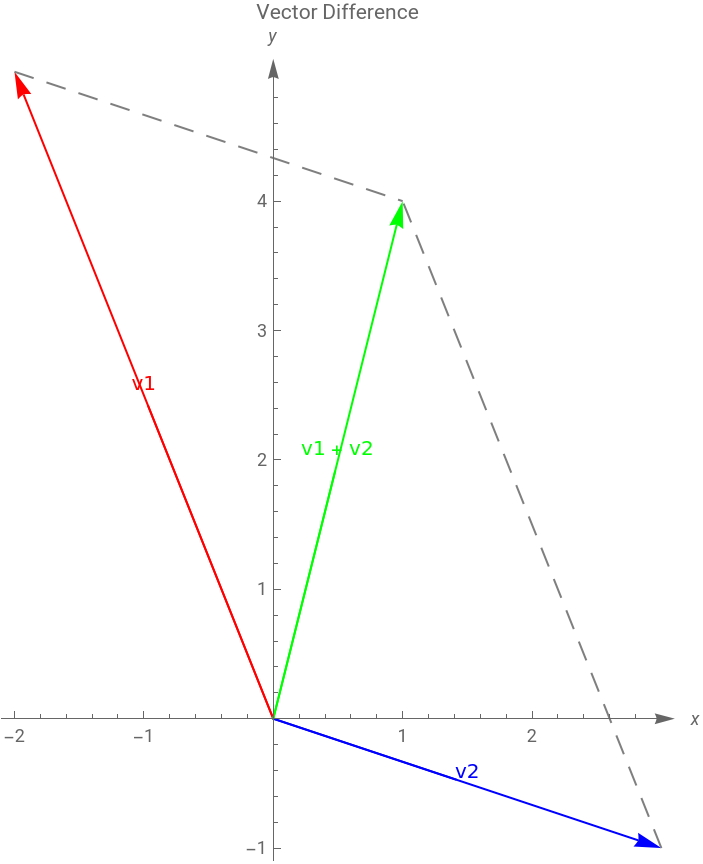
The sum of two vectors and is the vector .
v(a,b)
w(c,d)
v+w(a+c,b+d)
In[]:=
v1+v2
Out[]=
{1,4}
In[]:=
Show[Graphics[{Red,Arrow[{{0,0},v1}],Text["v1",v1/2,{0,-1}],Blue,Arrow[{{0,0},v2}],Text["v2",v2/2,{0,-1}],Green,Arrow[{{0,0},v1+v2}],Text["v1 + v2",(v1+v2)/2,{0,-1}],Dashing[{0.03,0.02}],Gray,Line[{v1,v1+v2}],Line[{v2,v1+v2}]}],Axes->True,AxesOrigin->{0,0},AxesLabel->{x,y},AxesStyle->Arrowheads[0.03],AspectRatio->Automatic,PlotRange->All,PlotLabel->"Vector Difference",Ticks->{Automatic,Automatic}]
Out[]=
◼
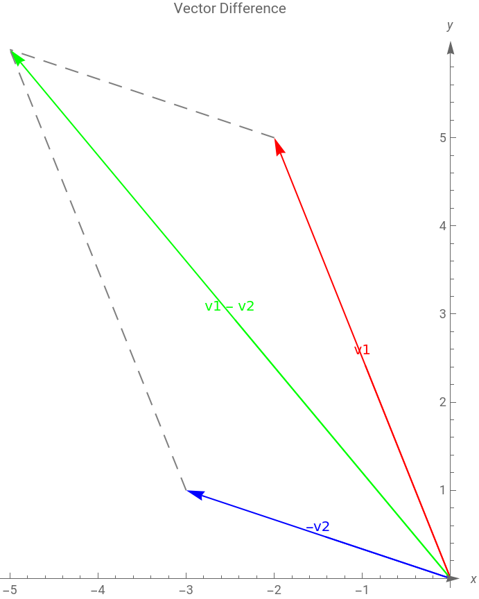
The vector difference of and in that order is .
v(a,b)
w(c,d)
v-w(a-c,b-d)
In[]:=
v1-v2
Out[]=
{-5,6}
In[]:=
Show[Graphics[{Red,Arrow[{{0,0},v1}],Text["v1",v1/2,{0,-1}],Blue,Arrow[{{0,0},-v2}],Text["-v2",-v2/2,{0,-1}],Green,Arrow[{{0,0},v1-v2}],Text["v1 - v2",(v1-v2)/2,{0,-1}],Dashing[{0.03,0.02}],Gray,Line[{v1,v1-v2}],Line[{-v2,v1-v2}]}],Axes->True,AxesOrigin->{0,0},AxesLabel->{x,y},AxesStyle->Arrowheads[0.03],AspectRatio->Automatic,PlotRange->All,PlotLabel->"Vector Difference",Ticks->{Automatic,Automatic}]
Out[]=
◼
The product of the vector by the scalar (real number) is .
v(a,b)
r
rv(ra,rb)
In[]:=
5*v1
Out[]=
{-10,25}
Example
Example
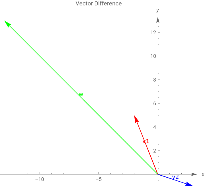
Findandplotandcompute
2-3
v
1
v
2
||2-3||
v
1
v
2
In[]:=
r=2;
In[]:=
r*v1
Out[]=
{-4,10}
In[]:=
s=3;
In[]:=
s*v2
Out[]=
{9,-3}
and
In[]:=
w=r*v1-s*v2
Out[]=
{-13,13}
In[]:=
Norm[w]
Out[]=
13
2
In[]:=
Show[Graphics[{Red,Arrow[{{0,0},v1}],Text["v1",v1/2,{0,-1}],Blue,Arrow[{{0,0},v2}],Text["v2",v2/2,{0,-1}],Green,Arrow[{{0,0},w}],Text["w",(w)/2,{0,-1}]}],Axes->True,AxesOrigin->{0,0},AxesLabel->{x,y},AxesStyle->Arrowheads[0.03],AspectRatio->Automatic,PlotRange->All,PlotLabel->"Vector Difference",Ticks->{Automatic,Automatic}]
Out[]=
3 - Dimensional Vectors
3 - Dimensional Vectors
Vector products
Vector products
Dot product
Dot product
The dot product of any two vectors of the same dimension can be done with the dot operation given as Dot[vector 1, vector 2]
Consider the vectors:
Cross product
Cross product
The cross product can be done on two vectors. It is important to note that the cross product is an operation that is only functional in three dimensions. The operation can be computed using the Cross[vector 1, vector 2] operation
Vector Angles
Vector Angles
The definition of a dot product yields
We can compute the angle between our two vectors :
Example
Example
Now, consider the following vectors
Addition
Addition
Subtraction
Subtraction
Linear combination of the vectors
Linear combination of the vectors
References
References
1
.James F. Hurley, 2002, University of Connecticut, Department of Mathematics, 196 Auditorium Road Unit 3009, Storrs CT 06269-3009. https://www2.math.uconn.edu/~hurley/math220/Mathematica_docs/VectPlot.pdf
3
.MATHEMATICA TUTORIAL Part 2.1: Vectors
https://www.cfm.brown.edu/people/dobrush/am34/Mathematica/ch1/vector.html
https://www.cfm.brown.edu/people/dobrush/am34/Mathematica/ch1/vector.html
CITE THIS NOTEBOOK
CITE THIS NOTEBOOK
Geometric and Algebraic Representations of Vectors
by Athanasios Paraskevopoulos
Wolfram Community, STAFF PICKS, October 10, 2023
https://community.wolfram.com/groups/-/m/t/3030841
by Athanasios Paraskevopoulos
Wolfram Community, STAFF PICKS, October 10, 2023
https://community.wolfram.com/groups/-/m/t/3030841