Introduction
Introduction
What is a bioreactor (Chemostat)?
What is a bioreactor (Chemostat)?
In[]:=
StringJoin[Riffle[Take[TextWords[WikipediaData["chemostat"]],67]," "]](*SourceWikipedia*)
Out[]=
A chemostat from chemical environment is static is a bioreactor to which fresh medium is continuously added while culture liquid containing left over nutrients metabolic end products and microorganisms is continuously removed at the same rate to keep the culture volume constant By changing the rate with which medium is added to the bioreactor the specific growth rate of the microorganism can be easily controlled within limits
In[]:=
WebImageSearch["Chemostat",1]
Out[]=
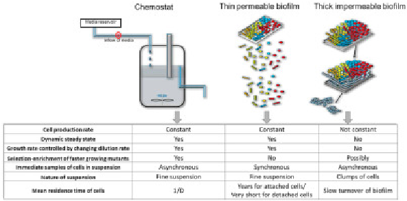
The chemostat is an experimental device invented in the 1950’ s, almost simultaneously, by Jacques Monod on the one hand, and by Aaron Novick and Leo Szilard on the other hand, which allows to study relationships between growth and environment parameters
Differential Equations modeling the biological reactions
Differential Equations modeling the biological reactions
Variables Definition
Variables Definition
dS
dt
S
in
dX
dt
S(t)
t
X(t)
t
S
in
D
-1
μ(S)
S
t
Two Main Types of models:
μ(S)
◼
Monod :
μ(S)+S
μ
max
S
K
s
◼
Haldane :
μ(S)+S+
μ
max
S
K
s
2
S
K
i
One Chemostat
One Chemostat
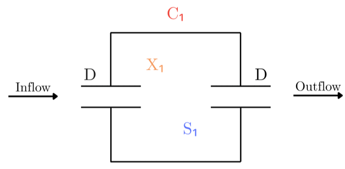
Definition of the Base Model: The standard chemostat differential equations
Definition of the Base Model: The standard chemostat differential equations
{S'[t]==(Sinput-S[t])-μ[S[t]]*X[t],X'[t]==μ[S[t]]*X[t]-X[t]}
Out[]=
{[t](Sinput-S[t])-X[t]μ[S[t]],[t]-X[t]+X[t]μ[S[t]]}
′
S
′
X
The first equation describes how the substrate concentration 𝑆(𝑡) changes over time by taking into account the fresh substrate that enters the chemostat ,as well as considering the substrate leaving with the outflow at the same time. It then subtracts to it all the number of bacterias that consume substrates for growth.
The second equation describes how the biomass concentration 𝑋(𝑡) (bacterias) changes over time, by acknowledging bacterial growth depending on substrate availability
minus the bacterias that are washed out of the reactor with the outflow
The second equation describes how the biomass concentration 𝑋(𝑡) (bacterias) changes over time, by acknowledging bacterial growth depending on substrate availability
minus the bacterias that are washed out of the reactor with the outflow
Monod’s law
Monod’s law
We first define μ(S), the bacterial growth rate, and solve the differential equations in order to compute and obtain a numerical solution for any set of parameters
In[]:=
μ[S_,k_,μmax_]:=μmaxClear[k,μmax]chemostat=ParametricNDSolveValue[{S'[t]==(Sinput-S[t])-μ[S[t],k,μmax]X[t],X'[t]==μ[S[t],k,μmax]X[t]-X[t],S[0]==S0,X[0]==X0},{S,X},{t,0,Tmax},{Sinput,,k,μmax,S0,X0,Tmax}]
S
k+S
Out[]=
ParametricFunction


We plot μ(S) , which represents the growth rate of the bacterias as a function of the substrate concentration:
In[]:=
Manipulate[Plot[μ[S,k,μmax],{S,0,10},PlotRange->{0,5},ImageSize->Large,PlotLabel->"μ(S)depending on S"],{{k,3.5},0.01,25},{{μmax,3.8},0.01,10},SaveDefinitions->True]
Out[]=


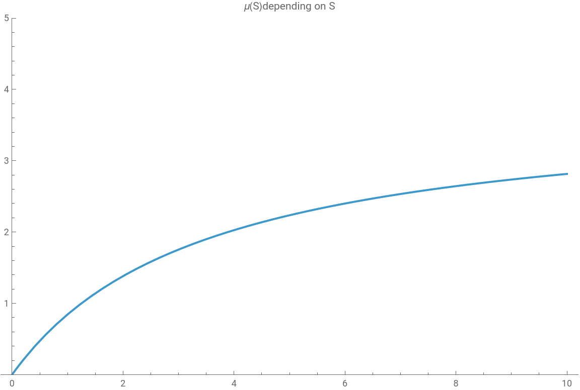
For very small 𝑆 the denominator 𝑘 + 𝑆 ≈ 𝑘 (k represents the half saturation level, and measures the affinity for the substrate, in other terms, how capable the cells are to consume substrate to grow efficiently).
Intuitively, if there' s barely any substrate, the bacterias are limited and can only grow slowly , unless k = 0, meaning that there is no gradual increase : as soon as you have any substrate, cells grow at their maximum possible rate.
While, as 𝑆 gets very large, the + 𝑘 becomes negligible compared to 𝑆, thus the fraction in Monod' s law approaches 1, and this means the growth rate levels off and never exceeds 𝜇max.
Intuitively, if there' s barely any substrate, the bacterias are limited and can only grow slowly , unless k = 0, meaning that there is no gradual increase : as soon as you have any substrate, cells grow at their maximum possible rate.
While, as 𝑆 gets very large, the + 𝑘 becomes negligible compared to 𝑆, thus the fraction in Monod' s law approaches 1, and this means the growth rate levels off and never exceeds 𝜇max.
We then plot both μ(S) and :
In[]:=
Manipulate[Row[{Show[Plot[{,μ[S,k,μmax]},{S,0,10},PlotLegends->{"","μ(S)"},PlotRange->{0,5},PlotStyle->{Purple,Orange},ImageSize->Small,PlotLabel->"Growth rate of X and Dilution rate"],Graphics[{PointSize[0.03],Red,Point[{Sinput,0}]}],Graphics[{Dashed,Red,Line[{{Sinput,0},{Sinput,5}}]}],Graphics[{PointSize[0.03],Orange,Point[{-((k)/(-μmax)),0}]}],Graphics[{Dashed,Orange,Line[{{-((k)/(-μmax)),0},{-((k)/(-μmax)),μ[-((k)/(-μmax)),k,μmax]}}]}]],Show[Plot[Evaluate[Comap[chemostat[Sinput,,k,μmax,S0,X0,Tmax],t]],{t,0,Tmax},PlotLegends->{"S","X"},PlotRange->{0,6},ImageSize->Small,PlotLabel->"Evolution of X and S"],Plot[{*k/(μmax-),Sinput-(k*)/(μmax-)},{t,0,Tmax},PlotStyle->{{Gray,Dashed}},PlotLabel->"Evolution rate"]]}],Row[{Button["Demo 1",{=2.5}],Button["Demo 2",{=3.5}]}],{{,2.5},0,5},{{Sinput,5},0,5},{{k,1},0,5},{{μmax,4},0,5},{{Tmax,10},1,20},{{S0,4},0,5},{{X0,1},0,5},ControlPlacement->Left,SaveDefinitions->True]
When the dilution rate exceeds the growth rate of the bacteria (which depends on substrate concentration), the system experiences a ‘washout’, meaning that the bacteria count eventually goes to 0.
Solution to find the equilibrium values:
Solution to find the equilibrium values:
Vector field plot and Graph plot of the dynamical system
Vector field plot and Graph plot of the dynamical system
Demo 1 simulates a situation where bacteria grows and substrate decreases until the system approaches a steady state (red lines show the theoretical equilibrium values). It highlights two solutions ( the trivial equilibrium , or also called the washout point, as well as the non trivial solution)
Demo 2 simulates a situation were their is no substrate in the feed, coming into the system, so bacterias consume the substrate that is initially within the system until both bacteria and substrate counts decrease towards 0. It shows the point of coordinates (0;0), where both substrate and bacteria levels approach 0
Demo 3 simulates a situation where bacterias are barely able to keep up with the outflow until experiencing complete washout.
The vector visually reflects what the plot has previously shown. It shows only 1 equilibrium → the system is washed out.
Demo 2 simulates a situation were their is no substrate in the feed, coming into the system, so bacterias consume the substrate that is initially within the system until both bacteria and substrate counts decrease towards 0. It shows the point of coordinates (0;0), where both substrate and bacteria levels approach 0
Demo 3 simulates a situation where bacterias are barely able to keep up with the outflow until experiencing complete washout.
The vector visually reflects what the plot has previously shown. It shows only 1 equilibrium → the system is washed out.
Haldanes’s law
Haldanes’s law
We define μ(S) once again, but with a different law modelising the bacterial growth rate, and solve the differential equations in order to compute and obtain a numerical solution for any set of parameters:
We plot μ(S) , now with Ks ( half-saturation constant: the substrate concentration at which the growth rate is half of its maximum), 𝜇0 ( the maximum specific growth rate: the maximum growth rate of the microorganisms when substrate is optimal) and 𝐾𝐼 ( inhibition constant: the substrate concentration at which growth starts to be inhibited due to excess substrate)
Solution to find the equilibrium values:
Solution to find the equilibrium values:
Demo 1 simulates a situation where their is only one positive root to the quadratic expression, so the Dilution rate plot only touches the growth rate plot in one point.
Demo 2 has a very odd point in the middle: which corresponds to the unstable equilibrium. This is explained by the stability of equilibria that comes originally from the Jacobian matrix of the system.
If Dynamic>0 the equilibrium is unstable. Biologically, it acts as a threshold, so if bacteria density 𝑋 is above it,the system goes to the stable positive equilibrium. However,if it’s below, the system collapses to washout.
Demo 0 simulates washout.
Demo 2 has a very odd point in the middle: which corresponds to the unstable equilibrium. This is explained by the stability of equilibria that comes originally from the Jacobian matrix of the system.
If Dynamic>0 the equilibrium is unstable. Biologically, it acts as a threshold, so if bacteria density 𝑋 is above it,the system goes to the stable positive equilibrium. However,if it’s below, the system collapses to washout.
Demo 0 simulates washout.
One Chemostat with two bacterias
One Chemostat with two bacterias
Two bacterias ‘ growth respecting the monod’s law
Two bacterias ‘ growth respecting the monod’s law
We define kX and kY (two different k variables with coefficients in order to differentiate their growth) and then plot the two growth functions and the dilution rate
We then solve the differential equations modeling the configuration where a chemostat contains two bacteria ( X and Y):
The vector plot shows three equilibrium points, each representing independently the trivial point ( if we set X, so the X bacteria count to 0), and the equilibrium points :Single-species equilibrium where X dominates ( with 𝑋>0,𝑌=0) and where Y dominates (𝑌>0,𝑋=0).
Furthermore, we can observe that one bacteria specie always finishes by dominating the other one reflecting the competitive exclusion principle: Both species initially grow while S is abundant.As they consume S, the concentration drops.The species with the lower 𝑆*still survives at this new lower S level.The other species cannot sustain growth (𝜇(𝑆)<𝐷)and is washed out.
Two bacterias' growth respecting the Haldane's law
Two bacterias' growth respecting the Haldane's law
Same as the simulation with Monod’s law, this model demonstrates once again the principle of competitive exclusion.
Two bacterias’ growth each respectively respecting Monod’s law and Haldane’s law
Two bacterias’ growth each respectively respecting Monod’s law and Haldane’s law
All three simulations are quite similar.
Two Chemostats with two bacterial species
Two Chemostats with two bacterial species
We use Monod’s law in order to avoid an abundance of parameters
The double chemostat system exploited here assumes that the first reactor has already reached its equilibrium values (S1*, X1*) before feeding into the second reactor, which creates a cascade effect where the second reactor' s dynamics depend on the steady - state output from the first .
The equations that allow for a steady state are a result of:The substrate entering from reactor 1 being equal to the substrate consumed by both microorganisms plus the substrate leaving the reactor,
and the X biomass entering from reactor 1 plus new X biomass produced by growth must equal the X biomass leaving the reactor
and also the Y biomass produced by growth must equal the Y biomass leaving the reactor
The equations that allow for a steady state are a result of:The substrate entering from reactor 1 being equal to the substrate consumed by both microorganisms plus the substrate leaving the reactor,
and the X biomass entering from reactor 1 plus new X biomass produced by growth must equal the X biomass leaving the reactor
and also the Y biomass produced by growth must equal the Y biomass leaving the reactor
Three chemostats (with double parralel reactors branched to a main chemostat),and two bacterias
Three chemostats (with double parralel reactors branched to a main chemostat),and two bacterias
In our model, X1 and Y1 are the populations of the two species in those first-stage chemostats. The effluents from both S1 (substrate in chemostat 1) and S2 feed into the third chemostat (S3), where both species (X2 and Y2, which is essentially the same as X1 and Y1, but with a slight modification in the variable name) can coexist and compete for the mixed substrate pool. X2 and Y2 represent the downstream populations of the two species in the final chemostat.
By simulating a more complex setup, determined by 7 differential equations, we observe more intricate dynamics, especially the coexistence of both X and Y bacterias:In the first stage, 𝑌 dominates in chemostat 1 (S1) and 𝑋 dominates in chemostat 2 (S2), since each grows best on its own substrate environment. Both effluents then feed into chemostat 3 (S3), so the two populations are introduced together with a mixed substrate pool. Because neither species completely washes out the other at this point — each has a continuous input flow from its upstream chemostat — both 𝑋 and 𝑌 can maintain positive growth
Coexistence of all four species occurs in the range of D where a vertical line intersects the points of all four different colors. ( even though some colors are covered by others, you can see by plotting separately there exists parameters for which we can obtain a perfect coexistence state)
Cyclic model (prey-predator configuration)
Cyclic model (prey-predator configuration)
IBM Model
IBM Model
The ODE approach(using differential equations to analyse chemostat environment) Treats substrate concentration 𝑠(𝑡)
s(t) and biomass densities 𝑥(𝑡),𝑦(𝑡) as continuous variables,Assumes well-mixed, large populations, no randomness. Moreover, growth and washout are smooth and predictable functions of time. This can be problematic because we consider the population by its whole, not by individual bacterias that make up the population. Thus, we used an IBM approach to observe ho an individual based model can simulate a similar situation ( here using the configuration of a chemostat, and 2 bacterias).On the other hand the IBM model is stochastic and discrete, constructed on a totally different structure. However, we do notice that the several IBM realizations tend towards the original ODE: thus reflecting Kurtz’s theorem: as population size → ∞, the stochastic master equation → deterministic ODE
s(t) and biomass densities 𝑥(𝑡),𝑦(𝑡) as continuous variables,Assumes well-mixed, large populations, no randomness. Moreover, growth and washout are smooth and predictable functions of time. This can be problematic because we consider the population by its whole, not by individual bacterias that make up the population. Thus, we used an IBM approach to observe ho an individual based model can simulate a similar situation ( here using the configuration of a chemostat, and 2 bacterias).On the other hand the IBM model is stochastic and discrete, constructed on a totally different structure. However, we do notice that the several IBM realizations tend towards the original ODE: thus reflecting Kurtz’s theorem: as population size → ∞, the stochastic master equation → deterministic ODE
CITE THIS NOTEBOOK
CITE THIS NOTEBOOK
Simulation of the chemostat: mathematical theory of microorganism cultures
by Loric Bobon
Wolfram Community, STAFF PICKS, August 31, 2025
https://community.wolfram.com/groups/-/m/t/3538166
by Loric Bobon
Wolfram Community, STAFF PICKS, August 31, 2025
https://community.wolfram.com/groups/-/m/t/3538166