This notebook series is designed to introduce selected dynamic economic models to both advanced undergraduate and graduate students. Economists have relied on a series of economic models to better understand the otherwise highly complex causal relationship among many economic variables. Dynamic economic models set up by systems of either difference or differential equations are particularly useful in tracing the change in the quantity of unknown economic variables (e.g., the capital stock, demand for labor, aggregate output, etc.) and their interactions over time.
This notebook series aims to help students better understand the depth, usefulness, and limitations of major existing micro and macroeconomic models by demonstrating how we can use Wolfram Mathematica to replicate and reconstruct the core ideas and find dynamic solution of the model.
The model introduced in this notebook series include, among others, (1) the cobweb model of the quantity and price adjustment, (2) Keynes’s aggregate demand model, (3) Hicks’s ISLM model, (4) Samuelson’s investment accelerator model, (5) Kalecki’s investment delay model, (6) the predator-prey interaction model, (7) the epidemic model, (8) Ricardo’s three dimensional business cycle model, (9) Marx-Goodwin business cycle and growth model, (10) Smith’s and Ricardo’s growth model, (11) the Harrod-Domar growth model, (12) the Solow growth model, (13) the RBC model, (14) Romer’s new growth model, and (15) the circuit of capital model.
The Cobweb model of supply and demand
Introduction
Introduction
The Cobweb model of supply and demand is one immediate extension from a static supply and demand model. Suppose that the producer-seller uses the price of a unit of product at t-1 when (s)he supplies the product on the market at time t. In this case, the supply equation becomes a function of the price of the product one time period earlier, and the supply and demand model is composed of one linear demand equation and one difference equation for supply. The solution to this model is no longer a pair of two numbers but instead becomes a function. The exact behavior of the solution curve of this function depends on the parameter and the initial value. This note presents the basic cobweb model of supply and demand and shows how we can find and visualize the solution curve.
The model structure
The model structure
The quantity demanded remains a negative function of a price of the product, whereas the quantity supplied is a positive function of the price of the product one time earlier.
Q[t]=d0-d1P[t]Q[t]=s0+s1P[t-1]
where all parameters d0,d1, s0 and s1 are positive constants. The parameter d1 is the price sensitivity of the quantity demanded, whereas s1 is the price sensitivity of the quantity supplied.
At equilibrium the two quantities equal with one another, which gives rises to the following linear first-order difference equation.
In[]:=
Clear[Q,P,d0,d1,s0,s1,t];Solve[d0-d1P[t]==s0+s1P[t-1],P[t]]
Out[]=
P[t]
d0-s0-s1P[-1+t]
d1
If the initial value of P[t], P[0] is given by P0, the analytical solution to this difference equation becomes:
In[]:=
RSolveP[t]==,P[0]==P0,P[t],t//Simplify
d0-s0-s1P[-1+t]
d1
Out[]=
P[t]
d0-d0+P0(d1+s1)+s0-1+
t
-
s1
d1
t
-
s1
d1
t
-
s1
d1
d1+s1
A numerical example 1
A numerical example 1
Suppose we have the following parameters and the initial value of P(t):
In[]:=
d0=4;d1=1.7;s0=0.5;s1=1.1;P0=1;
The numerical solution becomes:
In[]:=
RSolveP[t]==,P[0]==P0,P[t],t
d0-s0-s1P[-1+t]
d1
Out[]=
{{P[t]-0.25(-5.+1.)}}
t
(-0.647059)
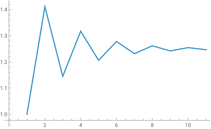
Using a built-in DiscretePlot [ ] function, we can draw a following graph that shows the behavior of the P[t]:
In[]:=
?DiscretePlot
Out[]=
In[]:=
DiscretePlot[-0.25`(-5.`+1.`),{t,0,10}]
t
(-0.6470588235294118`)
Out[]=
We can find and visualize the same solution curve using different Mathematica functions, RecurrenceTable [ ] and ListLinePlot[ ] and as follows:
In[]:=
d0=4;d1=1.7;s0=0.5;s1=1.1;P0=1;
In[]:=
?RecurrenceTable
Out[]=
In[]:=
sol1=RecurrenceTableP[t]==,P[0]==P0,P,{t,0,10}
d0-s0-s1P[-1+t]
d1
Out[]=
{1.,1.41176,1.14533,1.31773,1.20618,1.27836,1.23165,1.26187,1.24232,1.25497,1.24678}
In[]:=
?ListLinePlot
Out[]=
In[]:=
ListLinePlot[sol1]
Out[]=
A numerical example 2
A numerical example 2
Suppose this time that the producer’s supply response is changed, s1 = 1.9. Then the solution becomes:
In[]:=
d0=4;d1=1.7;s0=0.5;s1=1.9;P0=1;sol2=RecurrenceTableP[t]==,P[0]==P0,P,{t,0,10};ListLinePlot[sol2]
d0-s0-s1P[-1+t]
d1
Out[]=
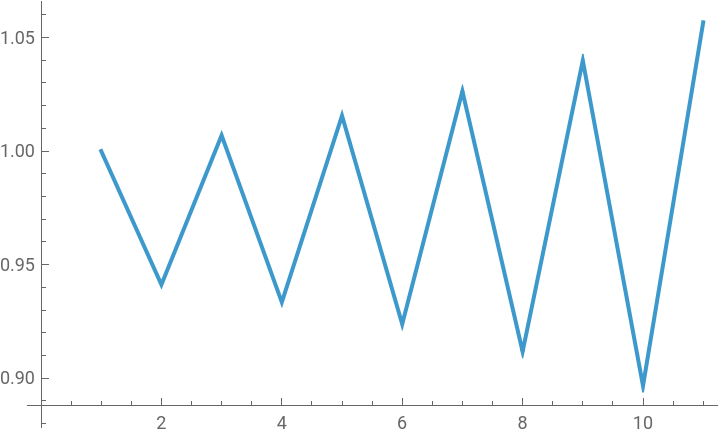
Instead of converging, the equilibrium price continue to diverge away from its notional steady state value.
Conclusion
Conclusion
The cobweb model of the price adjustment is one insightful extension of a simple supply and demand model. By introducing a time delay in the quantity supplied on the product market, the model shows how the equilibrium price changes over time (either converging to or diverge away from the steady state value), depending on the parameters and the initial value.
One can easily extend this model by introducing an additional time delays. For example, we can think of a possibility that the producer and supplier adjusts the price of the product based upon the market prices of the product observed in the past two time periods, instead of the price at time t-1. In this case, the supply equation and the resulting equilibrium condition yields a linear second-order difference equation.
We can also introduce series of inventory-workforce adjustment variables. If we assume that the producer’s sales is equal to the demand for this product and the producer wants to hold some positive inventory stock in order to meet the unexpected surge in the demand, we can successively derive various inventory variables such as the desired inventory stock, inventory coverage period, time to fill the inventory gap by engaging in active production activities, etc., and tie them to the dynamic supply and demand adjustment process. Since the supply and the inventory management requires this producer-seller to hire a desired number of workers (given the average capital-labor ratio), we can also introduce the desired workforce, actual workforce, and time delay for hiring new workers, etc., to construct a more comprehensive dynamic model. In this way, we can easily expand this simple cobweb model to account for the dynamic adjustment in both inventory stock and workforce.
Reference
Reference
Michael Hoy et al. Mathematics for Economics, The MIT Press: 2022, pp.752-754 and pp.798-802.
Ronald Shone, An Introduction to Economic Dynamics. Cambridge University Press: 2001, pp.27-35.
Srinivas Raghavendra and Petri T. Piiroinen, An Introduction to Economic Dynamics - Modelling, Analysis and Simulation, Routledge: 2023, pp.15-32.
CITE THIS NOTEBOOK
CITE THIS NOTEBOOK
Introduction to dynamic economic models: the Cobweb model of supply and demand
by Hee-Young Shin
Wolfram Community, STAFF PICKS, December 11, 2025
https://community.wolfram.com/groups/-/m/t/3587038
by Hee-Young Shin
Wolfram Community, STAFF PICKS, December 11, 2025
https://community.wolfram.com/groups/-/m/t/3587038