ORIGINAL ARTICLE: Jing B. Wang, Paul C. Abbott, Jim F. Williams; Visualizing atomic orbitals. Comput. Phys. 1 January 1996; 10 (1): 69–82. DOI: https://doi.org/10.1063/1.168561
Article Abstract: The Mathematica software package provides a range of tools for working with atomic systems. The symbolic tools include orthogonal polynomials and Clebsch-Gordan coefficients whilst the graphical capabilities cover polar plots; spherical plots; density plots; contour plots in two and three dimensions; and animation. These tools are applied to the manipulation and visualization of atomic orbitals.
INTRODUCTION
INTRODUCTION
The probability distribution of the electron charge cloud in an atom, namely the atomic orbital, often reveals crucial information in atomic physics. Visual representation of such orbitals is invaluable to researchers working in this field and also helps teaching atomic structures to physics or chemistry students. The atomic orbital concepts were discussed in detail by Berry and the cited papers therein, including several visualization devices. However, the newly developed symbolic package Mathematica provides a wider range of graphical tools (including polar plots, spherical plots, density plots, contour plots in two and three dimensions, and animation), which can be applied to help visualise the radial and angular behaviour of multi-dimensional systems.
Mathematica also has a wide range of built-in special functions appropriate for the analysis of quantum systems. Orthogonal polynomials — Legendre, Laguerre, Chebyshev, Hermite and Jacobi (corresponding to the Mathematica functions (x), (x), (x), (x), (x), and (x)) — arise when solving a wide class of eigenvalue and boundary value problems. The spherical harmonics, (θ,ϕ), are eigenfunctions of the angular part of the Laplacian operator (which is the quantum mechanical angular momentum operator).
P
n
a
L
n
U
n
T
n
H
n
(a,b)
P
n
m
Y
l
Clebsch-Gordan coefficients
arise in the study of angular momenta in quantum mechanics, and in other applications of the rotation group. These functions, taken together with the orthogonal polynomials and graphical tools, provide a powerful environment for the study of atomic systems. It is worth noting that these methods can be readily utilized in the studies of other multi-dimensional systems.As this article is not intended to be a tutorial on Mathematica, commands and syntax will not usually be explained. However, it is hoped that by showing a well-chosen set of examples, even readers unfamiliar with Mathematica will be able to follow the examples. The graphical output is placed immediately after its corresponding input command as it appears in Mathematica notebooks. Arbitrary units are used in these graphs.
1. NOTATION AND PREREQUISITES
1
. NOTATION AND PREREQUISITESThe quantity
Ω(r)r=
ψ n,l,m | pure basis state | ψ n,l,m |
ψ n,l | coherently mixed state | ψ n,l ∑ m c m ψ n,l,m |
where
ψ
n,l,m
R
n,l
m
Y
l
2
r
represents the probability of finding an electron in the volume element . The spherical harmonics, (θ,ϕ), give the angular distribution of the atomic orbitals and (r) is the corresponding radial distribution.
r
m
Y
l
R
n,l
In the following, the general spherical harmonic will be denoted using the Mathematica shorthand (θ,ϕ). For example,
m
Y
l
1
Y
2
-sin(θ)cos(θ)
1
2
15
2π
ϕ
Although it is a built-in operation, complex conjugation, required to yield real-valued charge densities, is more easily achieved using a replacement rule:
In[]:=
*
exp_
For example,
*
1
Y
2
Out[]=
-sin(θ)cos(θ)
1
2
15
2π
-ϕ
We make use of the Notation package to define custom input and output notations.
In[]:=
<<Notation`
In[]:=
Symbolize[]
′
j
2. ANGULAR DISTRIBUTION OF ATOMIC ORBITALS
2
. ANGULAR DISTRIBUTION OF ATOMIC ORBITALS1. Pure states ψnlm(r)
1
. Pure states ψ
nlm
For pure basis states, (r), the angular distribution:
ψ
n,l,m
ang
Ω
l,m
2
(θ,ϕ)
m
Y
l
is axially symmetric with respect to the azimuthal angle . In this case, PolarPlot can provide a complete view of the atomic orbitals.
ϕ
After defining the angular distribution function:
In[]:=
Ω
l_,m_
m
Y
l
*
m
Y
l
individual charge densities can be immediately examined, e.g.,
Ω
3,2
Out[]=
105(θ)(θ)
4
sin
2
cos
32π
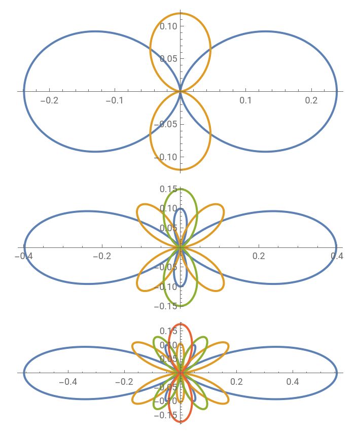
Here are plots of the atomic orbitals for the states , .
l=1,2,3
m=0,…,l
GraphicsColumn@TablePolarPlotEvaluateTable(θ),{m,0,l},{θ,0,2π},PlotRangeAll,{l,1,3}
Ω
l,m
Out[]=
In[]:=
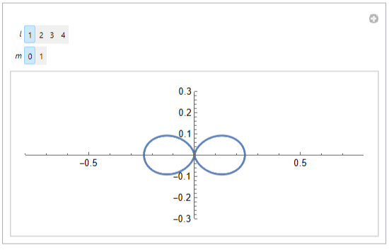
ManipulatePolarPlotEvaluate(θ),{θ,0,2π},AspectRatioAutomatic,PlotRange{{-0.8,0.8},{-0.3,0.3}},{l,Range[4]},{{m,0},Range[0,l],ControlTypeSetterBar},SaveDefinitions->True
Ω
l,m
2. Mixed states ∑mcmψnlm(r)
2
. Mixed states ∑
m
c
m
ψ
nlm
For coherently mixed states
ψ
nl
∑
m
c
m
ψ
nlm
R
nl
∑
m
c
m
m
Y
l
the angular probability distribution is
ang
Ω
l
2
(θ,ϕ)
∑
m
c
m
m
Y
l
In this case, the charge cloud is no longer axially symmetric and its distribution is a function of both and . Three-dimensional plots are thus required to depict the structure of the coherently mixed atomic orbitals.
θ
ϕ
In general, the expression
ω
l
l
∑
m=-l,2
a
m
b
m
m
Y
l
where () are the amplitude ratio (relative phase) of each state, can be evaluated in Mathematica using:
a
m
b
m
In[]:=
ω
l_
ω
l
l
∑
i=0
c
〚i+1,1〛
c
〚i+1,2〛
l-2i
Y
l
The argument to needs to be a list of pairs. The general angular charge distribution then reads:
c
{,}
a
m
b
m
In[]:=
Ω
l_
ω
l
*
ω
l
where the core of this expression is the product of (c)(θ,ϕ) with its complex conjugate, (c). The other operations, Expand, ComplexExpand, and Factor, are used to simplify the expression to a human readable form.
ω
l
ω
l
*
(θ,ϕ)
As an example, for the general -state wavefunction can be obtained from the mixed state consisting of , :
P
l=1
m=±1
ψ
P
Ω
1
1 | 0 |
a | b |
Out[]=
3(θ)(-2acos(b-2ϕ)+1)
2
sin
2
a
8π
and then plot the orbitals for the states with parameters :
{a=0.1,b=0}
In[]:=
Manipulate[SphericalPlot3D[Evaluate[(a,b)],{θ,0,π},{ϕ,0,2π},BoxRatios1,PlotRange0.5,MeshFalse,AxesFalse,BoxedFalse,SphericalRegionTrue],{{a,0.8},0,1},{{b,π/2},0,π},SaveDefinitions->True]
ψ
P
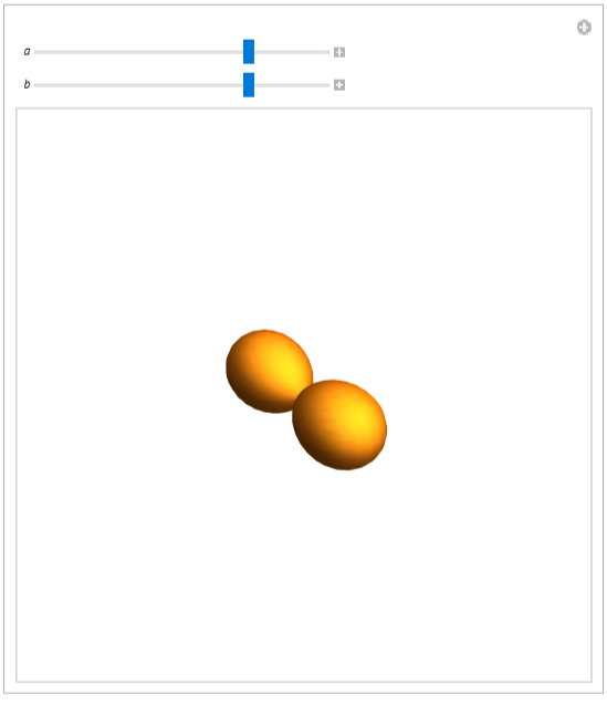
Note that the full range of ϕ was not shown to highlight the structure of the orbital.
Choosing the parameters arbitrarily as
one can produce a three-dimensional graph:
We clear the values assigned in this section.
Due to the interaction between the intrinsic magnetic dipole moment of the electron (spin) and the internal magnetic field of the atom (orbital angular momentum), the atomic charge density evolves with time. Animation provides views of such dynamic effects. Taking the spin-orbit (L-S) coupling into account, we obtained the time-dependent charge density function for a mixed state:
where
implemented in Mathematica as
are the so-called state multipoles and the corresponding time evolution factor is
implemented in Mathematica as
The time-dependent charge density function becomes
This can be plotted using the commands,
This command displays a sequence of graphics objects in succession and thus simulates the time evolution of the orbitals. Alternatively, here is an array of animation frames:
We clear the values assigned in this section.
For the hydrogen atom the radial wavefunction in atomic units is
where
The radial wavefunction is easily defined:
The radial distribution function,
then becomes
We have so far plotted separately the angular and the radial distribution functions of various atomic orbitals. However, these pictures are incomplete on their own and one needs to imaginatively assemble the angular and the radial plots in order to obtain a complete picture of the charge distribution in three-dimensional space.
Mathematica's DensityPlot is then adequate for showing the detailed distribution of the two-variable function, where the lighter region indicates higher charge density:
Defining a set of rules to transform from spherical polar to Cartesian coordinates:
the distribution in Cartesian coordinates is easily obtained:
Finally, for a general coherent mixture of several magnetic states
the total charge density distribution is a function of three variables (r,θ,ϕ):
can be plotted using ContourPlot3D. Here are the surfaces for the contour levels 0.0003, 0.0015, and 0.003.
and for the molecular charge density of the bonding,
and antibonding orbitals,
To see these orbitals in three dimensions, we also plot their contour surface at an arbitrary level of 0.005:
This article has demonstrated the capabilities of Mathematica for analyzing and visualizing atomic systems. The interplay between symbolic and graphical methods yields a tool that is more powerful than the sum of its parts and one that can be superior to special purpose visualization tools because of its flexibility.
Even for readers that have never used a computer algebra system, an examination of some of the code fragments presented above — say those implementing the radial wavefunctions for hydrogenic atoms or the triple integral of spherical harmonics — illustrates that implementing some quite complicated formulae in Mathematica is straightforward and transparent and, hence, less likely to contain or conceal an error. One of the goals of object oriented programming is to implement high-level structures. All of the computations in this article could, of course, be done in FORTRAN or C (or C++). However, in general, the physicist or chemist does not want to write packages for computing orthogonal polynomials, spherical harmonics, Clebsch-Gordan coefficients or basic graphical tools. Of course, there exists libraries of public domain and commercial software which, when linked together, can provide equivalent capabilities. But, since all these capabilities, along with general symbolic manipulation, are built-in to Mathematica it can be seen to be an ideal tool for a wide range of analysis of atomic and molecular systems.
REREFENCES
REREFENCES
1. R.S. Berry, J. Chem. Ed. 43, 283 (1966)
2. S. Wolfram, Mathematica: A System for Doing Mathematics by Computer (Addison-Wesley, Reading, 1991)
3. A.R. Edmonds, Angular Momentum in Quantum Mechanics (Princeton, New Jersey, 1974)
4. B.H. Bransden and C.J. Joachain, Physics of Atoms and Molecules (Longman, UK, 1989)
5. K. Blum, Density Matrix Theory and Applications (Plenum: New York, 1981)
6. M. Abramowitz and I.A. Stegun, Handbook of Mathematical Functions (Dover, New York, 1972)
7. J.F. Shriner and W.J. Thompson, Computers in Physics, 7, 144 (1993)
CITE THIS NOTEBOOK
CITE THIS NOTEBOOK
Visualizing atomic orbitals
by Jingbo Wang, Paul C. Abbott, and Jim F. Williams
Wolfram Community, STAFF PICKS, October 10, 2023
https://community.wolfram.com/groups/-/m/t/3031372
by Jingbo Wang, Paul C. Abbott, and Jim F. Williams
Wolfram Community, STAFF PICKS, October 10, 2023
https://community.wolfram.com/groups/-/m/t/3031372