Consider the hyperbolic plane , realized in the Poincaré half-plane model. We can interpret this as the upper half-plane together with the Riemannian metric .
2
(x,y)∈:y>0
2
=+
2
s
1
2
y
2
x
2
y
In other words, if , then =+=(+).
U=+,V=+∈
u
1
∂
∂x
u
2
∂
∂y
v
1
∂
∂x
v
2
∂
∂x
T
(x,y)
2
〈U,V〉
(x,y)
u
1
v
1
2
y
u
2
v
2
2
y
1
2
y
u
1
v
1
u
2
v
2
Therefore, if is the Levi-Civita connection associated with this Riemannian metric, one can check that, using the notation and , X=Y, Y=X=-X, Y=-Y.
∇
X=
∂
∂x
Y=
∂
∂y
∇
X
1
y
∇
X
∇
Y
1
y
∇
Y
1
y
Now, consider the curve for some fixed >0. This is a horocycle centered at . It’s parametrized by arclength since , which is a unit vector since .
α(t)=(t,)
y
0
y
0
y
0
y=∞
α'(t)=X
y
0
∥X===1
y
0
2
∥
〈X,X〉
y
0
y
0
(t,)
y
0
y
0
2
y
0
2
y
0
If we want to parallel translate a tangent vector at, say, , then we get a vector field along the curve which satisfies the differential equation . Here is the covariant derivative along the curve .
W
0
α(0)=(0,)
y
0
W(t)=a(t)X+b(t)Y
0==W(t)=XW(t)
DW
t
∇
α'(t)
∇
y
0
D
t
α
Expanding this out a bit, we see that .
0=XW(t)=X(a(t)X+b(t)Y)=[a'(t)X+a(t)X+b'(t)Y+b(t)Y]=a'(t)-X+b'(t)+Y
∇
y
0
∇
y
0
y
0
∇
X
∇
X
y
0
b(t)
y
0
a(t)
y
0
X
Y
a'(t)-=0b'(t)+=0.
b(t)
y
0
a(t)
y
0
If we want to be the unit vector Y∈, then we have the initial conditions .
W
0
y
0
T
(0,)
y
0
2
a(0)=0,b(0)=
y
0
Mathematica will happily solve this initial value problem:
In[]:=
DSolvea'[t]-==0,b'[t]+==0,a[0]==0,b[0]==,{a,b},t
b[t]
y
0
a[t]
y
0
y
0
Out[]=
aFunction{t},Sin,bFunction{t},Cos
t
y
0
y
0
t
y
0
y
0
Here’s a visualization showing the resulting parallel fields when =,1,2:
y
0
1
2
In[]:=
GraphicsTableBlack,Thickness[.005],InfiniteLine[{{0,y0},{1,y0}}],Orange,TableArrow{y0t,y0},{y0t,y0}+y0Sin,Cos,{t,-4π,4π,2π/30},{y0,{1/2,1,2}},PlotRange->{{-π,π},{-.1,4}},Axes->True,Ticks->{Range[-π,π,π],Range[0,4]}
t
y0
t
y0
Out[]=
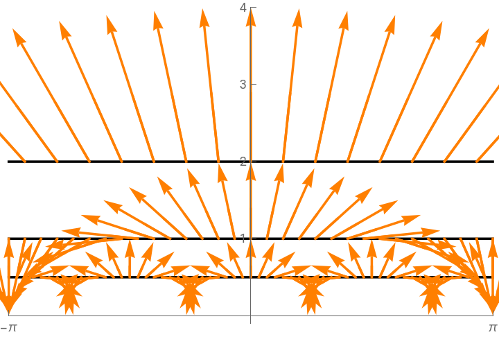
A parallel vector field is always pointing in the same direction from the perspective of someone inside the manifold, so the way to interpret this is that a person traversing the curve is constantly turning to the left to stay on . This makes sense: the geodesics (which are the straight paths) are vertical lines and semi-circles centered at points on the -axis, so at each point going “straight ahead” would mean walking along the semi-circle tangent to at that point. So to stay on you have to turn (to the left!) away from that semi-circle.
α(t)=(t,)
y
0
y
0
α
x
α
α
Now we start to turn this into an animation. In all of what follows, we’ll use = (based on the value of this parameter that I thought gave good results in the final animation).
y
0
2
3
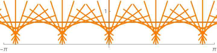
The arrows look a little bit too mathy, so let’s show the corresponding line field instead:
In[]:=
Withy0=,GraphicsBlack,Thickness[.005],InfiniteLine[{{0,y0},{1,y0}}],Orange,TableLine{y0t,y0}-y0Sin,Cos,{y0t,y0}+y0Sin,Cos,{t,-2π,2π,2π/30},PlotRange->{{-π,π},{-.1,4/3}},Axes->True,Ticks->{Range[-π,π,π],Range[0,1]}
2
3
t
y0
t
y0
t
y0
t
y0
Out[]=
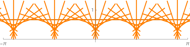
Which we can animate:
In[]:=
Withy0=,AnimateGraphicsBlack,Thickness[.005],InfiniteLine[{{0,y0},{1,y0}}],Orange,TableLine{y0s,y0}-y0Sin,Cos,{y0s,y0}+y0Sin,Cos,{s,-2π+t,2π+t,2π/30},PlotRange->{{-π,π},{-.1,4/3}},Axes->True,Ticks->{Range[-π,π,π],Range[0,4]},{t,0,2π/30},SaveDefinitions->True,AnimationRunning->False
2
3
s
y0
s
y0
s
y0
s
y0
Out[]=
Let’s make this look a little more pleasant by shortening the lines, getting rid of the axes and underlying curve, and using some different colors (taken from this ColorHunt palette):
In[]:=
Withy0=,cols=RGBColor/@{"#384B70","#FCFAEE"},AnimateGraphicsCapForm["Round"],Thickness[.0025],cols[[1]],TableLine{y0s,y0}-Sin,Cos,{y0s,y0}+Sin,Cos,{s,-2π+t,2π+t,2π/60},PlotRange->{{-2,2},{0,4/3}},Background->cols[[2]],ImageSize->600,{t,0,2π/60},SaveDefinitions->True,AnimationRunning->False
2
3
y0
8
s
y0
s
y0
y0
8
s
y0
s
y0
Out[]=
To produce the final animation, we’re going to transform the curve (which remember was a horocycle centered at ) to a horocycle centered at a finite point on the -axis.
α
y=∞
x
Recall that the Cayley transform maps the upper half-plane model to the Poincaré disk model, and of course its inverse (z)= goes the other way:
f(z)=
z-
z+
-1
f
1+z
1-z
In[]:=
Cayley[z_]:=;CayleyInverse[z_]:=I;
z-I
z+I
1+z
1-z
And then we get back into the upper half-plane model by applying the inverse of the Cayley transform:
Here’s our line field from before, fed through this transformation (strictly speaking, I should really be applying the differential of the map to the vector field, but that requires more work):
Here’s the code to produce the actual GIF:
CITE THIS NOTEBOOK
CITE THIS NOTEBOOK
Parallels (parallel translation along a horocycle)
by Clayton Shonkwiler
Wolfram Community, STAFF PICKS, June 3, 2025
https://community.wolfram.com/groups/-/m/t/3473522
by Clayton Shonkwiler
Wolfram Community, STAFF PICKS, June 3, 2025
https://community.wolfram.com/groups/-/m/t/3473522